
Links of the dimensional chain. Dimension chains
A dimensional chain is a set of interconnected dimensions that determine the relative position of the axes and surfaces of one part or several parts in a product, located in a certain sequence along a closed contour and directly affecting the accuracy of one of the contour dimensions.
Each dimensional chain consists of the constituent links (sizes) of the chain and the master link (size).
The closing size is the size obtained last in the process of machining a part or assembling a unit, the magnitude and accuracy of which depend on the magnitude and accuracy of all other dimensions of the chain, called components. According to the relative position of the dimensions, dimensional chains are divided into linear, planar and spatial.
Dimensional chains are called linear, the links of which are parallel to each other.
Dimensional chains are called planar, all or part of the links of which are not parallel to each other, but located in one or more parallel planes
Dimensional chains are called dimensional chains, all or part of the links of which are not parallel to each other and are located in non-parallel planes
Dimensional chains are called angular, all the links of which are angular values. Signs of the constituent dimensions of an angular chain are often non-perpendicularity, non-parallelism of axes and surfaces, and similar errors in the relative position of surfaces and axes of parts
Increasing are the constituent dimensions, with an increase in which the closing dimension increases.
Reducing are called constituent sizes, with an increase in which the closing size decreases.
The size of the assembly dimensional chain, which determines the functioning of a unit or mechanism, is called the initial (functional) size (clearance, interference, amount of movement of the part, etc.). During assembly, this dimension is usually the closing dimension.
Limit deviations of sizes are assigned, mainly, guided by the following rules:
the tolerance is assigned to the body of the part;
for enclosing dimensions, the deviation is assigned to "+";
for the dimensions covered, the deviation is assigned in "-";
for other sizes, deviations are assigned symmetrically - "±" (deviations in absolute value are equal to half of the tolerance).
When calculating dimensional chains distinguish between direct and inverse problems.
The direct task is to determine the tolerance and maximum deviations of the constituent dimensions according to the given nominal dimensions of all chain links and the given maximum deviations of the original (closing) link.
The inverse problem is to determine the nominal value, tolerance and maximum deviations of the closing size for the given nominal dimensions and maximum deviations of the constituent links.
The direct problem associated with dimensional chains is solved when designing new structures of parts, assemblies and machines (design calculations).
The inverse problem is solved in cases when in the drawings the tolerances for the constituent dimensions are established by the designer, based on structural, technological and economic considerations and it is required to check their compliance with the tolerance of the closing link (verification calculations).
Both direct and inverse problems of dimensional analysis can be solved by the method of complete interchangeability; the theoretical-probabilistic method and other methods providing incomplete interchangeability.
Plane and spatial dimensional chains are calculated using the same methods as linear ones. It is only necessary to bring them to the form of linear dimensional chains. This is achieved by projecting the dimensions of a flat chain in one direction, usually coinciding with the direction of the closing dimension, and a spatial chain in two or three mutually perpendicular axes.
In dimensional analysis and synthesis of machine structures, methods are chosen to achieve the accuracy of the closing link, due to the methods of solving dimensional chains. The methods and techniques are self-contained and include the following.
The method of complete interchangeability is a method in which the required accuracy of the closing link of the dimensional chain is achieved in all cases of its implementation by including the constituent links without selecting, selecting or changing their values. To ensure complete interchangeability, dimensional chains are calculated in a maximum-minimum manner, taking into account only limit deviations links of the dimensional chain and their most unfavorable combinations using the system of additive tolerances. With such tolerances, their impact on production costs is significant. Providing the specified limit deviations in this case leads to a sharp increase in cost, and therefore calculations of the economically optimal accuracy are necessary.
The method of incomplete interchangeability is used when the required accuracy of the closing link of the dimensional chain is achieved with some risk by including the constituent links in it without the participation of other methods. In this case, overlapping tolerances are allowed, and the assembly can be carried out using the methods of group interchangeability, regulation, fitting, relying on the theoretical and probabilistic calculation method. The probabilistic method limits the production of defective products to a small allowable limit using a system of overlapping tolerances based on a random selection of parts.
With the method of group interchangeability, the required accuracy of the closing link of the dimensional chain is achieved by including in the dimensional chain of the component links belonging to the respective groups into which they are previously sorted. The choice of method presents an economic problem and implies additional production costs. Sorting parts increases the cost of new measuring technology and attracts expensive inspection machines. The labor costs of controllers are increasing. Warehousing costs are increasing due to the additional costs of storing sorted parts.
In the control method, the required accuracy of the closing link of the dimensional chain is achieved by changing the value of the compensating link without removing material from the compensator. The role of the compensator is usually performed by a special link in the form of a gasket, an adjustable stop, a wedge, etc. In this case, for all other dimensions of the chain, parts are processed according to extended tolerances that are economically acceptable for given production conditions. The disadvantages of this method include an increase in the number of parts in the machine, which complicates the design, assembly and operation.
In the fitting method, the required accuracy of the closing link of the dimensional chain is achieved by changing the value of the compensating link by removing a certain layer of material from the compensator according to the left allowance. Methods of joint processing of parts are used and with a large volume of work performed, with high accuracy it is automated.
The tasks of calculating dimensional chains include the following.
The synthesis problem (direct) is one at which the parameters of the closing link are set (nominal value, permissible deviations and tolerances) and it is required to determine the parameters of the constituent links.
The analysis problem (inverse) is a problem in which the parameters of the constituent links are known and it is required to determine the parameters of the closing link.
Taking into account the factors affecting the change in the links of the dimensional chain over time, two problems are solved - static and dynamic.
The essence of calculating the dimensional chain is to establish tolerances, maximum deviations, coordinates of their midpoints, nominal dimensions of all links.
By the type of tasks in the solution of which the circuits are involved, they are divided into design, technological and measuring.
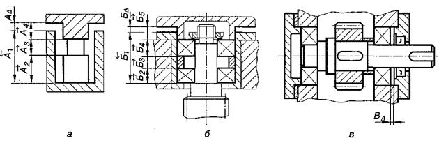
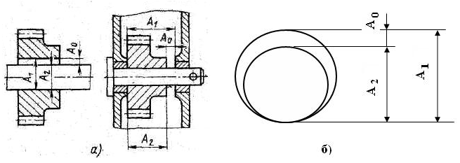
Designed dimensional chains solve the problem of ensuring accuracy in design. They establish a relationship between the dimensions of a part in a product. In fig. 9.1 shows examples of assembly dimensional chains.
In fig. 9.1, a an elementary assembly dimensional chain is presented, which solves the problem of ensuring the accuracy of mating two parts. In Figure 9.1, b an assembly chain is also shown, which solves the problem of ensuring the perpendicularity of surface 2 to axis 1, which is necessary for locating the rolling bearing.
Rice. 9.1 Examples of assembly dimensional chains.
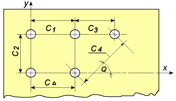
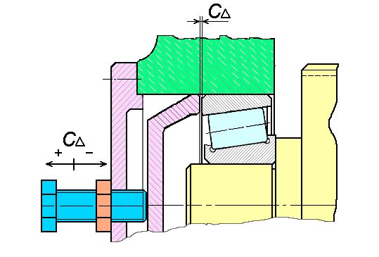
Technological dimensional chains solve the problem of ensuring accuracy in the manufacture of machines. They establish a relationship between the dimensions of the parts on different stages technological process. In fig. 9.2, a shows a part with dimensions that should be maintained during manufacture. The sequence for obtaining dimensions is shown in Fig. 9.2, b, c, d... On the basis of the proposed processing route, a technological dimensional chain was built (see Fig. 9.2, d). When processing a part, the dimensions are maintained C 1, C 2, C z and the size WITHΔ is obtained automatically.

Rice. 9.2. Principles of constructing design dimensional chains
Before building a dimensional chain, you should identify the closing link, which, for example, determines the normal functioning of the mechanism. The size or maximum deviation of the closing link is assigned or calculated based on the operating conditions and / or the required accuracy.
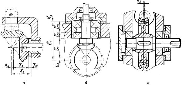
For example, the size and maximum deviations of the closing link A Δ are taken as such that would ensure free rotation of the gearwheel with the minimum possible displacement along the axis. The mismatch of the top of the pitch cone of the bevel gear with the axis of rotation of the bevel gear (Figure 9.5, a, b) determined by the degree of accuracy gear wheels, and its limit values are in accordance with the relevant standard. It is only necessary to establish between which parts the size of the master link is located, and then connect these parts with a chain of dimensions.
For example, in Fig. 9.3, b master link size B Δ stands between the axle and the end of the gear wheel; in fig. 9.5, a A Δ stands between the axis of the hole in the body and the top of the pitch cone of the bevel wheel, etc.
Let's consider the most typical options for assembly dimensional chains *. The first type of dimensional chains is shown in Fig. 9.3, the second is in Fig. 9.4., The third - in fig. 9.5.

Rice. 9.3. The first type of dimensional chain.
Rice. 9.4. The second type of dimensional chain.
Rice. 9.4. The third type of dimensional chain.
When constructing dimensional chains, one should be guided by their main properties:
the circuit must be closed;
the size of any link in the assembly chain must refer to elements of the same part; an exception is the closing link, which always connects elements of different parts;
the chain must be carried out in the shortest possible way, that is, the part with its elements must enter into the dimensional chain only once.
Basic relationships of dimensional chains
The dimensional chain is always closed. Based on this property, there is a relationship that links the nominal dimensions of the links. For flat dimensional chains with nominal links, it has the following form:
![]() (9,1)
(9,1)
where: n and p- the number of respectively increasing and decreasing links in the dimensional chain. To determine the dependence that connects the tolerances of the links in the dimensional chain, we first find the largest value of the closing link:
 (9.2)
(9.2)
then smallest value:
 (9.3)
(9.3)
Subtracting from (9.2) (9.3) we obtain:
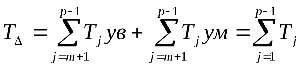
where: m- the number of links in the dimensional chain, including the master link.
Methods for solving dimensional chains
Complete interchangeability method. A method in which the required accuracy of the closing link of the dimensional chain is obtained for any combination of sizes of the constituent links. In this case, it is assumed that all links with limiting values can simultaneously appear in the dimensional chain, and in any of the two most unfavorable combinations (all increasing links with upper limiting dimensions, and decreasing ones with lower ones, or vice versa). Such a calculation method that takes these unfavorable combinations into account is called the maximum-minimum calculation method. .
Incomplete Interchangeability Method. This is a method in which the required accuracy of the closing link of the dimensional chain is obtained not with any combinations, but with a previously determined part of the combinations of the sizes of the constituent links.
The assembly is carried out without fitting, adjustment and selection of links.
The method is based on the assumption that the combination of the actual sizes of the constituent links in the product is random, and the probability that all the links with the most unfavorable combinations will be in one product is very small.
This method of calculation, which takes into account the scattering of sizes and the probability of their various combinations, is called the probabilistic method of calculation. In other words, the method allows a small percentage of products in which the closing link will go beyond the tolerance range. At the same time, the tolerances of the dimensions that make up the chain are expanded, and thereby the cost of manufacturing the parts is reduced.
The task of the calculation is to assign tolerances to the component links that correspond to the same degree of accuracy.
Fit method. This is a method in which the required accuracy of the closing link of the dimensional chain is achieved by changing the size of the compensating link by removing the metal layer from the compensator. Its essence lies in the fact that the tolerances for the constituent links are assigned according to economically acceptable qualifications, for example, according to the 12-14th qualifications. The resulting excess stray field at the closing link during assembly is eliminated by the compensator.
Control method using a fixed compensator
This is a method in which the required accuracy of the closing link of the dimensional chain is achieved by changing the compensating link without removing the metal layer.
Its essence lies in the fact that the excess of the dissipation field of the closing link is eliminated by selecting a compensator from a number of compensators made in advance with different sizes.
The meaning of the calculation is to determine the smallest number of expansion joints in the kit.
The meaning of the calculation is to determine the allowance for fitting, sufficient to compensate for the excess of the limit values of the closing link and, at the same time, the smallest one to reduce the amount of fitting work.
The role of the compensator is usually played by the part that is most accessible when disassembling the mechanism, simple in design and inaccurate, for example, gaskets, spacer washers.
Topic 6 Fundamentals of technical measurements. Dimension chains
The closing links of the dimensional chain are not directly performed but are the result of the execution, including the manufacture of all other links that make up the dimensional chain. Any dimensional chain has a master link and the constituent links of the dimensional chain. Each dimensional chain consists of constituent chain size links and a master size link.
Share your work on social media
If this work did not suit you at the bottom of the page there is a list of similar works. You can also use the search button
Dimension chains
One of the most effective methods for calculating the geometric parameters of the constituent parts of structures is the method of dimensional chains. The method allows the calculation of tolerances and deviations of geometric parameters or to check the correctness of their purpose to ensure the collection and performance of products.
The use of methods for calculating dimensional chains makes it possible to reduce both time and material costs at the stage of technical preparation and production of structures, improve the quality and shorten the terms of processing products, their design and technological documentation. Each dimensional chain has one master link. Such links are called closing links because in the process of assembling a product or when processing elements of individual parts, they close a real dimensional chain. The closing links of the dimensional chain are not directly performed, but are the result of the execution (including manufacturing) of all other links that make up the dimensional chain. The methods used to achieve the accuracy of the closing link, i.e. methods for calculating dimensional chains are shown in Figure 1.
Any dimensional chain has a master link and the constituent links of the dimensional chain. From the given methods for calculating dimensional chains, the "method of complete interchangeability" can be considered the basic one, on the basis of which the basic definitions and dependencies are obtained. Consideration of other methods after mastering the "method of complete interchangeability" becomes less difficult.
Figure 1. Methods for ensuring the accuracy of the closing link
Basic definitions and classification of dimensional chains
Dimensional chain is called a set of interconnected dimensions that determine the relative position of the axes and surfaces of one part (detailed dimensional chain, Fig. 2) or several parts in a product (assembly dimensional chain, Fig. 3), located in a certain sequence along a closed loop and directly affecting the accuracy of one from the outline dimensions.
Each dimensional chain consists of the constituent links (sizes) of the chain and the master link (size). Geometric diagrams eliminate the possibility of errors and simplify the task of identifying dimensional chains, especially with complex ladders.
Closing size(A Δ ; fig. 2, 3, 4) is the size obtained last in the process of machining a part or assembling a unit, the magnitude and accuracy of which depend on the magnitude and accuracy of all the other dimensions of the chain, called components (A1, A2 ... An-1; Fig. 2, 3).
The main typical closing links of dimensional chains include:
- gaps and tightness in the mates of parts;
- protrusions and overlaps of elements of some parts relative to others;
- symmetry of surfaces;
- the engagement of the surfaces of some parts relative to others;
- the alignment of the cylindrical surfaces of one or more parts;
- the distances between the surfaces of parts, which determine the beginning and end of the impact of one part on another.
The classification of the links of the dimensional chains of the dimensional chains is shown in table 1.
According to the relative position of the dimensions, dimensional chains are divided into linear, planar and spatial.
Linear dimensional chains are called, the links of which are located parallel to each other (Fig. 2, 3)
Plane dimensional chains are called, all orsome of the links of which are not parallel to each other, but located in one or more parallel planes (Fig. 4).
Spatialdimensional chains are called, all or part of the links of which are not parallel to each other and are located in non-parallel planes.
Corner dimensional chains are called, all links of which are angular values. Signs of the constituent dimensions of the angular chain are often deviations from perpendicularity, deviations from parallelism of axes and surfaces, and similar errors in the relative position of surfaces and axes of parts.
Classification of links of dimensional chains
Table 1
|
Definition |
Examples of |
|
|
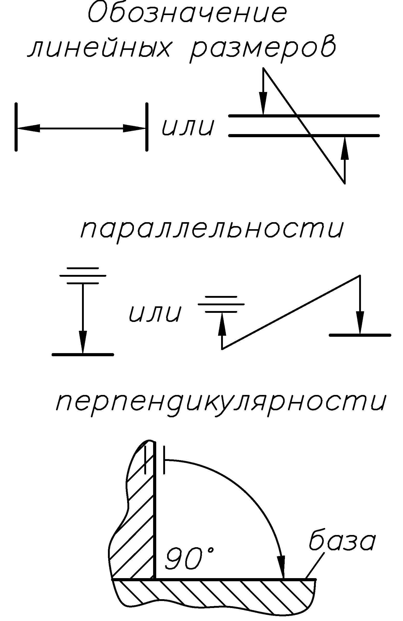
Link |
One of the dimensions that form a dimensional chain. On the diagrams of dimensional chains, the links are conventionally designated: linear dimensions - with a double-sided arrow; parallelism and perpendicularity - one-sided arrow with the direction of the arrow point to the base |
|
|
Closing |
The link of the dimensional chain, which is the initial one when setting the problem. For example, when designing, based on the service purpose of the mechanism, technical requirements are established ( limiting dimensions) to clearance A∆ - the closing link |
|
|
The link of the dimensional chain, resulting from the last as a result of solving the problem. For example, when assembling a gearbox, gear 2 and shaft 3 are installed in its housing 1. The last link of the dimensional chain is the gap A∆ - closing link |
|
|


Continuation of table. one
|
Constituent |
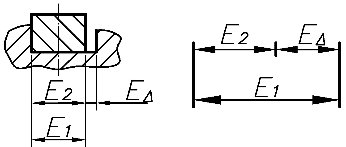
A link in a dimensional chain, functionally linked to the closing link. For example, links E 1 and E 2 dimension chain E |
|
|
Augmenting |
A constituent link of a dimensional chain, with an increase in which the closing link increases. For example, a link in a dimensional chain |
|
|
Reducing |
A constituent link of a dimensional chain, with an increase in which the closing link decreases. For example, a link in a dimensional chain |
|
|
Compensating |
A constituent link of a dimensional chain, by changing which the required accuracy of the closing link is achieved. For example, link A To - spacer ring for dimension chain A |
|


Rice. 2. Dimensional chain of the part
Rice. 3. Dimensional chain of the unit
Rice. 4. Plane dimensional chain
Table 2 shows the classification of dimensional chains.
table 2
Types of dimensional chains
|
Chain |
Definition |
|
Technological |
Dimensional chain that provides the required distance or relative rotation between the surfaces of the manufactured product when performing an operation or a series of assembly operations, processing, when setting up a machine or when calculating intertransition dimensions |
|
Design |
Dimensional chain that defines the distance or relative rotation between surfaces or surface axes of parts in an item |
|
Measuring |
Dimensional chain that occurs when determining the distance or relative rotation between surfaces, their axes or forming surfaces of a manufactured or manufactured product |
|
Linear |
Dimensional chain, the links of which are linear dimensions |
|
Corner |
Dimensional chain, the links of which are angular dimensions |
|
Flat |
Dimensional chain, the links of which are located in one or more parallel planes |
|
Spatial |
Dimensional chain, the links of which are located in non-parallel planes |
Increasing the constituent dimensions are called, with an increase in which the closing dimension increases.
Reducing the constituent dimensions are called, with an increase in which the closing dimension decreases.
For example, it is enough to add some small value to the size ( see fig. 4) , with the constancy of the remaining dimensions of the chain (here it is only), so that F ∆ decreased. If, leaving unchanged, add, then the closing F ∆ will increase.
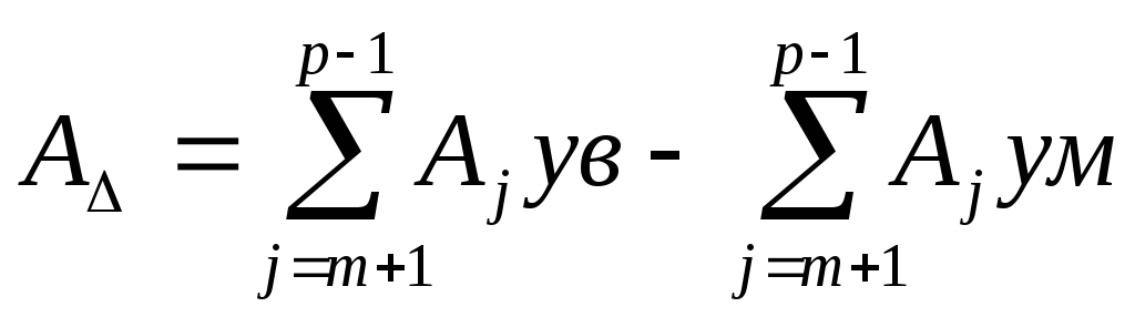
Given the division of sizes into increasing and decreasing, it is not difficult to write down the equation of the dimensional chain in denominations
A Δ = A i uv - A i um (1)
where in the dimensional chain:
m - the number of increasing sizes, (A i uv),
p - the number of reducing sizes (A i mind).
Total nominal sizes of the constituent links, taking into account the closing one, will be: n = m + p +1
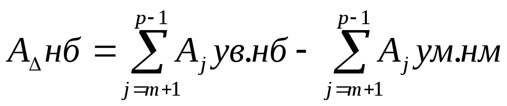
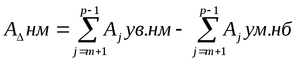
The limiting values of the dimensions of the closing link are determined by the equations, which logically follows from expression (1) and the definitions of increasing and decreasing sizes:
= - (2)
= - (3)
where: , - the largest and smallest limiting dimensions of the closing link;
, , - the largest and smallest limiting dimensions of the links.
The closing size tolerance is calculated as the difference between the largest (2) and the smallest (3) values of the closing size, that is, it is enough to add the last two equations and get
TA Δ = T A i (4)
where: TA Δ - closing size tolerance;
T A i - component size tolerance;
n –1 - the number of constituent links of the dimensional chain, without the closing one.
In general, for the dimensions of the dimensional chain A the ratio is true:
TA Δ = ││ T A i (5)
where: = gear ratio, n Is the number of chain links.
If the analysis of circuits with parallel links is carried out, then:
for increasing sizes = + 1,
for downsizing=- 1.
The parameter is most needed when formalizing the solution of problems, for example, when programming.
Limit values of the constituent dimensions and the closing linkin case the dimensions are specified by nominal values and deviations, they are determined by the formulas:
A i + ES i
A i + EI i
А Δ + ES Δ (6)
А Δ + EI Δ, (7)
where: А i, А Δ - the nominal values of the components and the closing size,
ES i, EI i, ES Δ, EI Δ - the upper and lower deviations of the components and the closing size.
We use the equation
=
Let us write it down taking into account the above definitions of the limiting values
A Δ + ES Δ = (A i uv + ES i uv) - (A i um + EI i um)
Substitute on the left side of the equation
A Δ = A i uv - A i um
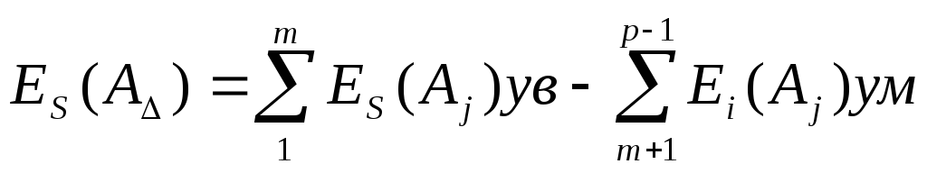
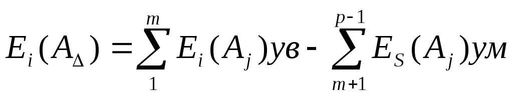
The upper and lower deviations of the closing size in this case are determined by the equations of the dimensional chain in deviations:
ES Δ = ES i uv - EI i um (8)
EI Δ = EI i uv - ES i um, (9)
where: ES i uv, EI i uv, ES i um, EI i um - the upper and lower deviations of the increasing and decreasing constituent links of the dimensional chain.
When solving a number of problems on dimensional analysis, it is more convenient to determine the upper and lower deviations of the closing size by the formulas throughthe coordinate of the middle of the tolerance zone:
ES Δ = Δ 0 A Δ + (10)
EI Δ = Δ 0 А Δ -, (11)
where: Δ 0 А Δ - T А Δ - the tolerance for the closing link, determined by the formula (5).
The coordinate of the middle of the tolerance field of the closing link is determined by the equation of the midpoints of the tolerance fields of the dimensional chain:
Δ 0 A Δ = Δ 0 A i uv - Δ 0 A i um, (12)
where: Δ 0 A i uv, Δ 0 A i um - coordinates of the middle of the tolerance field of the constituent links of the dimensional chain, determined by the dependence:
Δ 0 А i = (ES i + EI i) / 2
Taking into account expressions (11) and (12), the upper and lower deviations of the closing size are determined by the formulas:
ES Δ = (Δ 0 A i uv - Δ 0 A i um) + (13)
EI Δ = (Δ 0 A i uv - Δ 0 A i um) - (14)
It is known that the tolerance value of each component size is determined by the formula:
TA i = a i ∙ i i,
where: a - accuracy coefficient; i i = 0.45+ 0.001A i avg - unit of tolerance.
But it should be assumed that all the constituent links of the chain are of the same level of accuracy, which allows us to write:
a 1 = a 2 = a 3 = a 4 =… = a n-1 = a = const
Then :
TA i = a (0.45+ 0.001A i avg),
A i av - the average size of the range of sizes.
Considering equation (5) TAΔ = T A i,
Or
TA Δ = a ∙ i 1 + a ∙ i 2 + ... a ∙ i n-1 = a ∙
now we can write:
If initially in the dimensional chain some dimensions were with given tolerances (for example, bearing dimensions, etc.), then equation (5) will take the form:
Here k is the number of dimensions with specified tolerances. Now the final equation for the accuracy factor will be:
(15)
Having determined the accuracy factor, you can calculate the tolerances as T A i = a i i , but it is more rational to choose tolerances according to the nearest quality according to the tolerance table. In the case of the same dimensions of the constituent links or the dimensions that are in the standard range of dimensions, where “ i »Invariable for the interval, the formula is simplified
Or T A i = TA∆ / (n -1) (16)
As you can see, a single tolerance was obtained for all sizes. This method is simple, but essentially indicative and therefore is used mainly only for preliminary assignment of tolerances of constituent dimensions.
Dimensional tolerances are assigned as for the main shaft and the main hole, i.e. for those who increase in "+" and those who decrease in "-", with the exception of the linkage. For a linking dimension, the position of the tolerance is determined by one of the equations connecting the parameters of the closing dimension and the components, with the remaining parameters assigned.
The given dependences are valid for the method of complete interchangeability (MPV), where an equiprobable distribution of the resulting sizes is assumed. In other words, when shooting at a round target with aiming at the middle of the target, the probability of hitting "1" and "10" is the same, which is not entirely true.
Probability-theoretic method (TVM)
The probabilistic-theoretic method (TVM) is based on probabilistic distribution curves and, as a result, uses slightly different formulas (here we give without derivation). The presented dependencies provide for an equiprobable distribution and a risk coefficient of 0.27%.
…………………………(17)
…………………………(18)
The value of the tolerance of the linking dimension in the TBM is determined by the dependence
…………………………(19)
It is not difficult to see from the formulas that for TVM the tolerances will be wider than for MPV
Compensation method
In the control method, the accuracy of the closing link of the dimensional chain is achieved by changing the size of the compensating link without removing material from the compensator.
Movable expansion joints are devices or individual parts, due to the adjustment of which, achieved by moving or turning, the required size of the closing link is provided (Fig. 5).
Fixed expansion joints are, for example, replaceable gaskets, rings, bushings, washers, etc., installed during assembly until the required accuracy of the master link is achieved. Rationally prepare sets of expansion joints of the same or stepped thickness (Fig. 6).
Rice. 5. Movable expansion joint
Rice. 6. Fixed expansion joint
Movable compensators are divided according to the continuity of regulation into compensators with periodic regulation (threaded, wedge, eccentric, etc.) and compensators with continuous regulation, as a rule, automatic regulation of the technological process. By design, all types of expansion joints are divided into groups that compensate for linear or angular dimensions. The calculation of the parameters of dimensional chains is carried out by the maximum-minimum method or the probabilistic method.
The disadvantages of the regulation method include: incomplete interchangeability, some complication of the design by the introduction of a constructive compensator and the complication of the assembly due to the need to carry out the adjustment. The method has found wide application for ladder chains with high requirements for the accuracy of the closing links and a not so high level of accuracy of the constituent links.
The parameters of the constituent links of the dimensional chain with the control method are assigned in accordance with technologically and economically acceptable production conditions. The required compensation value TA To achieved by regulation using the types of compensators discussed above.
Let us write the equation
By adopting technologically and economically feasible extended tolerances, we can obtain
Introducing Ak and T A to can ensure equality
With the probability-theoretic method
To ensure the required accuracy of the closing link in the control method, the size of the minimum step of the compensators should not exceed the tolerance of the closing link:
With equality can be determinedrequired number of compensation steps
The resulting value of N determines the required number of gaskets with a certain margin.
At the stages of production and operation of the structure, it becomes necessary to solve inverse problems, when the parameters of the closing link are calculated according to the known (specified) parameters of all the constituent links of the dimensional chain. At the design stage, inverse problems are solved in order to verify the correctness of the solution of direct problems.
In the fitting method, the required accuracy of the closing link of the dimensional chain is obtained by removing a layer of material from the compensator to achieve the size of the compensating link. To do this, the compensating link of the compensator part enters the assembly with a predetermined allowance, which is removed by machining methods to achieve the required value of the closing link. This method allows you to establish economically viable tolerances for all components of the links in the dimensional chain. However, it should be noted that it is used only in individual and small-scale production. The disadvantages of the method include the rise in the cost of assembly and the increased labor intensity of assembly work, as well as the complication of planning and supplying the product with spare parts.
To master the theoretical dependencies, we will try to solve the dimensional chain of a simple knot using various methods.
Selective assembly
The essence of selective assembly is that the connection parts are manufactured with technologically feasible and economically feasible tolerances. The manufactured parts are measured and sorted into groups according to actual dimensions. The assembly of connections is carried out according to the groups of the same name.
Selective is called the assembly of products from parts previously sorted into groups according to their actual sizes. This method is used for various connections, including when solving dimensional chains and is also called the method of group interchangeability. Selective assembly allows you to increase the accuracy of the closing link of the dimensional chain without increasing the processing accuracy of the constituent links. It is possible to reduce the manufacturing accuracy of the component links of the assembly and by selective assembly to obtain the required closing size tolerance. C assembling of nodes is made from the groups of the same name. In some cases, mass production without selective assembly is generally impossible. For example, rolling bearings, critical tightness threads, precision piston groups, diesel fuel pumps, and other high-precision products can only be obtained through selective assembly.
Selective assembly is used:
In order to improve the accuracy of the closing dimension without reducing the tolerances on the parts that form the assembly;
In order to expand processing tolerances while maintaining the specified accuracy of the closing dimension.
Main advantageselective assembly - reducing costs and obtaining the required mating accuracy, the achievement of which is technologically difficult or impossible.
Flaws selective assembly:
Additional costs for measuring parts, sorting, marking, storage;
Incomplete (group) interchangeability is provided.
Work in progress occurs as a result of a different number of parts in the sorting groups of the same name.
Rational use in large-scale and mass production.
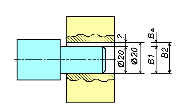
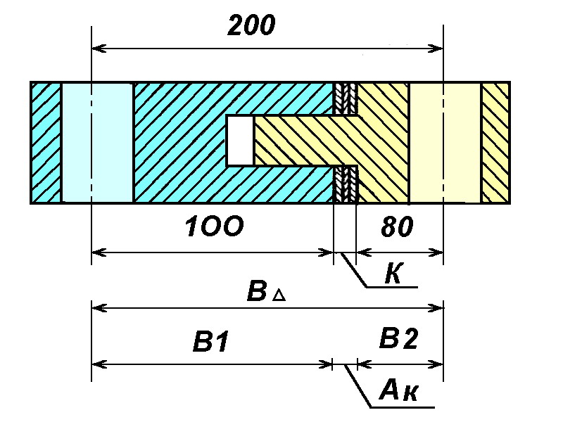
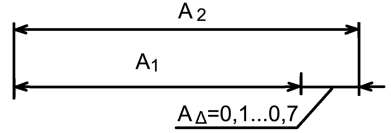
Example: must be manufactured to be assembled with the specified clearance.
![]()
Let's select the dimensional chain of the knot:
where n = 3, number of sizes
m = 1, increasing
n = 1, decreasing
Closing tolerance
TA ∆ = ES ∆ - EI ∆ = 0.7-0.1 = 0.6
Component tolerance
TAi =
Tai = T 1 A 2 = 300 μm
A 2 increasing, A 1 reducing. For A 2 we assign a tolerance to the body from zero and therefore A 2 = 20 + 0.3, for linking we will take A 1 according to the equation ES ∆ = -
ES ∆ = ESA 2 - EIA 1; EIA 1 = ESA 2 - ES ∆
EIA 2 = 0.3-0.7 = -0.4mm
ESA 2 = EIA 2 + TA 2 = -0.4 + 0.3 = -0.1 mm
Then A 2 =
a) The assembly conditions of the assembly have changed and it is necessary to obtain TA∆ = 300 μm.
You can order a new batch of parts with tighter tolerances.
But without making parts again, you can divide the batch into 2 groups:
A 1 = 20 A 1 = 20 TA ∆ = 300 μm
A 2 = 20 A 2 = 20 TA ∆ = 300 μm
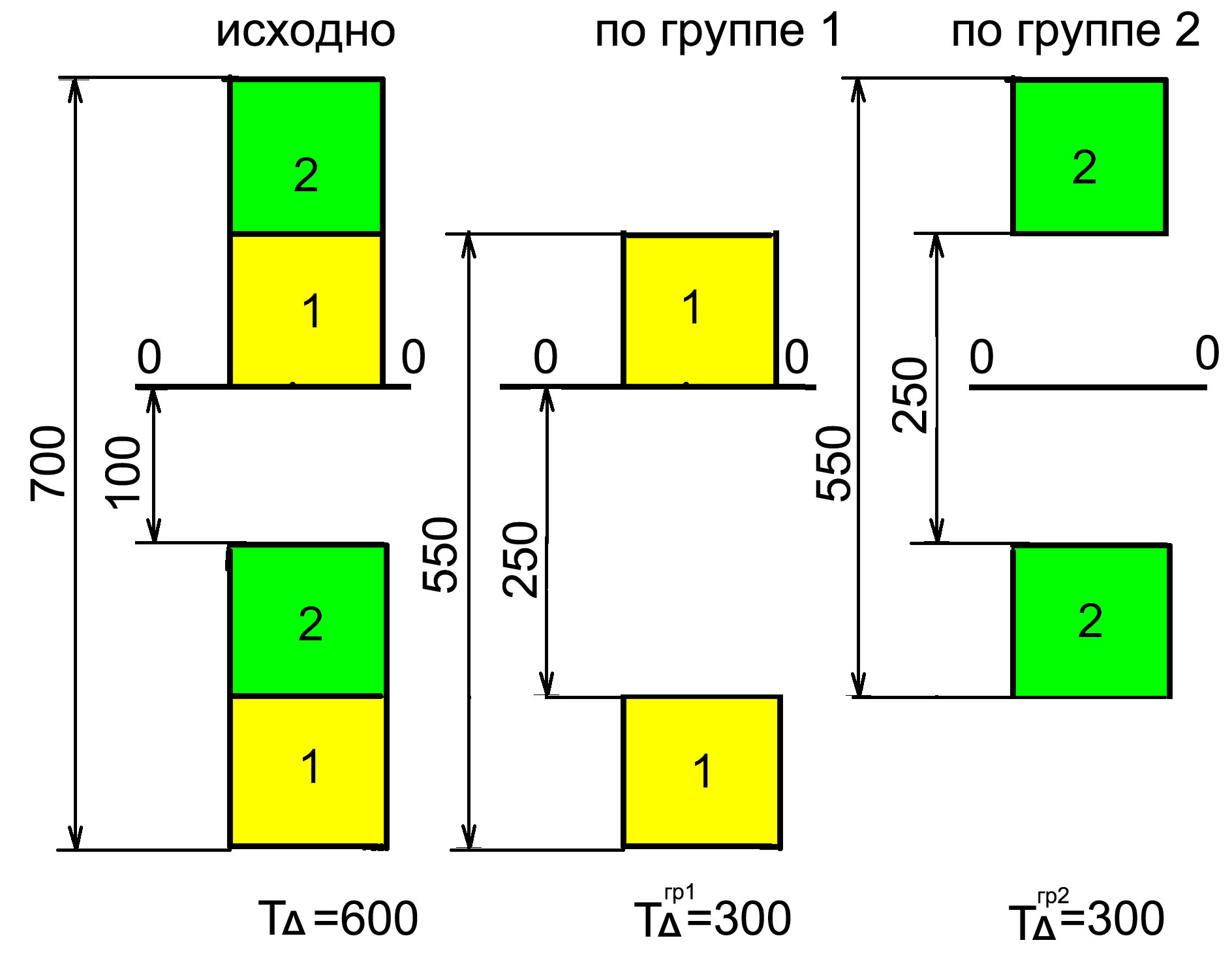
This solution was obtained on the assumption that the number of shafts and holes in groups is the same, which is not always the case with small-scale production, mass production allows you to practically collect 100% of the products.
b) the production conditions have changed and do not allow the manufacture of a product with TA ∆ = 0.6 mm. In this case, you can make a node with TA ∆ = 1.2 mm, and then, similarly dividing a series of parts into 2 groups, get the assembly TA ∆ = 0.6 mm.
Examples of solving problems of dimensional chains by various methods
Exercise :
For the knot in the first figure, carry out a comparative calculation of the dimensional chain using various methods.
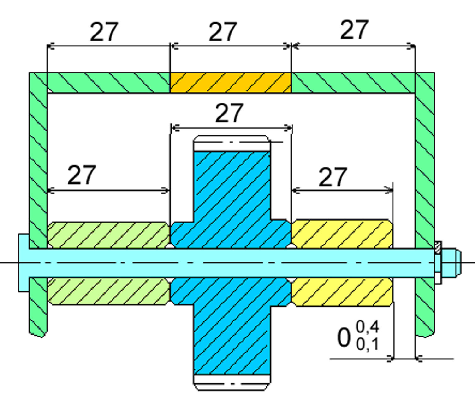
Drawing. Node 1.
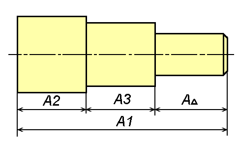
Let's select the dimensional chain from the node:
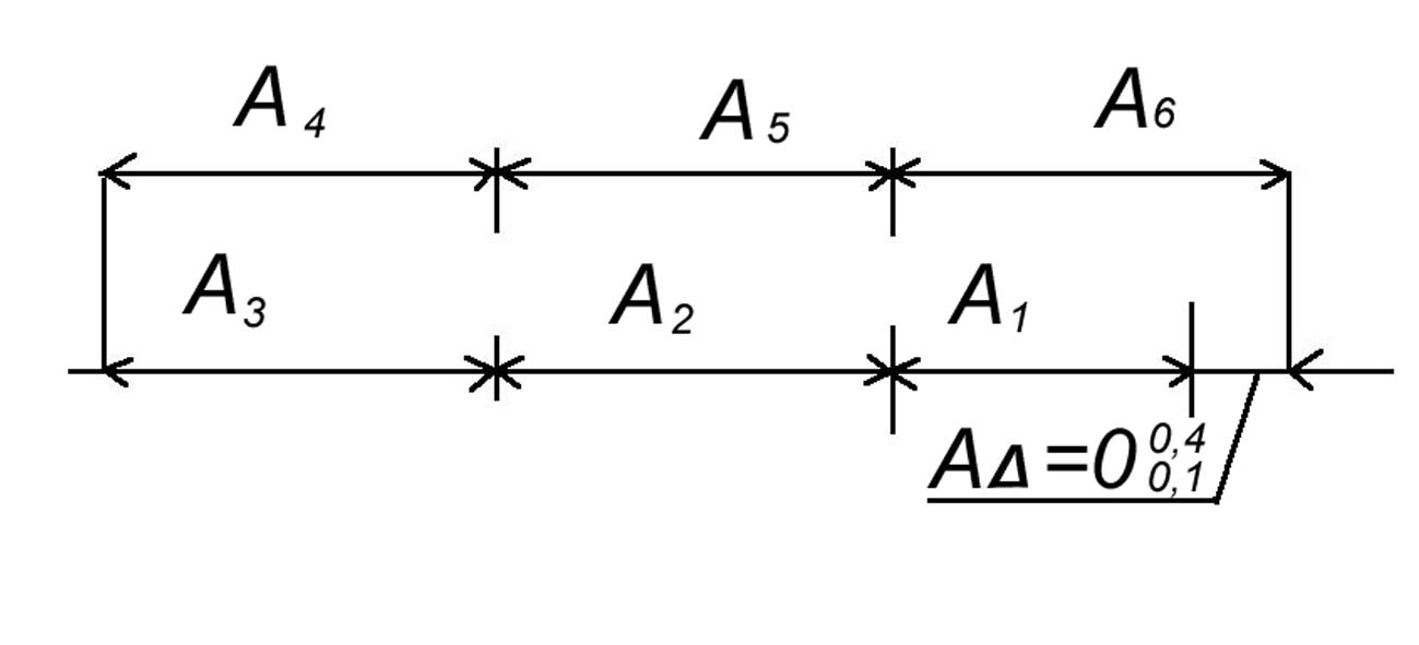
Drawing. RC-A
Total sizes in a dimensional chain n = 7, n = m + p,
where: m -increasing, p -decreasing
Increasing dimensions A 4, A 5, A 6, reducing dimensions A 1, A 2, A 3
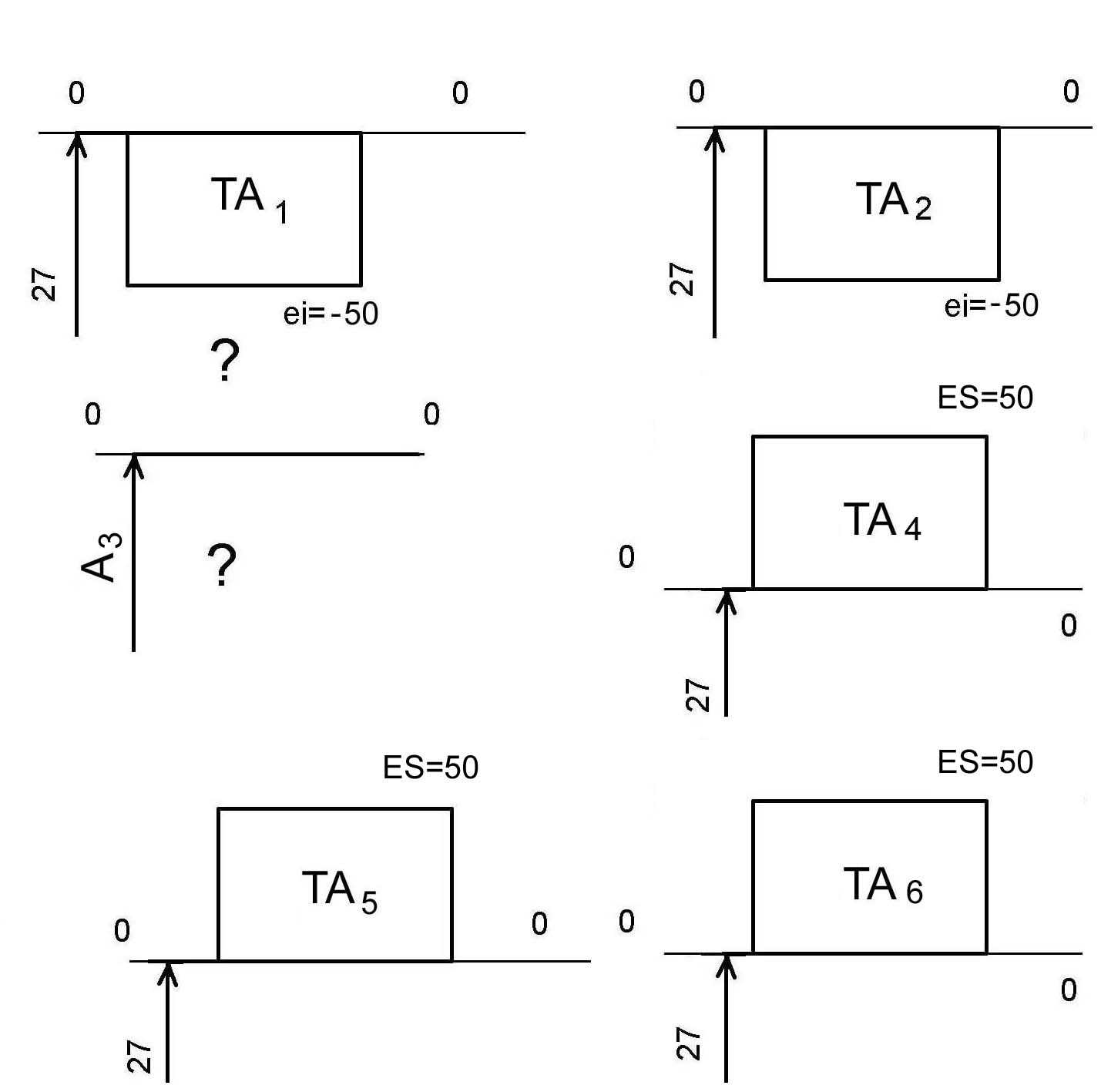
By the method of equal tolerances
Let's apply the formulas:
TA i = TA D / (n-1), TA i = 300 μm / (n-1) = 50 μm
Let's use the equation:
=
Having chosen as a linking size, we take a decreasing one, we get:
=
Let us graphically represent the position of the tolerances, taking them into the body of the part for all sizes, except for the link:
Drawing. Fields-A
Let's find its smallest value:
26,850
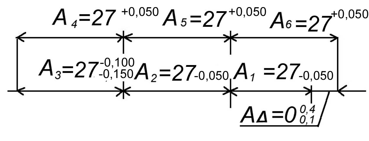
Drawing. RC-A with deviations
In an assembly, tolerances can be graphically represented as:
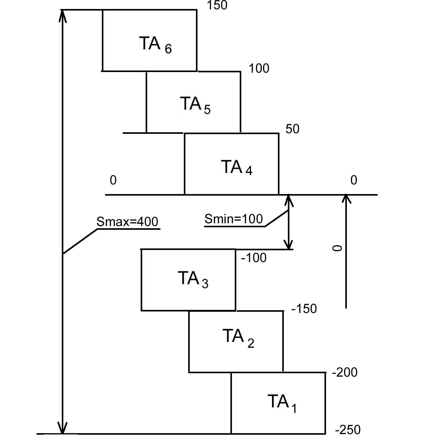
Drawing. Graphic chain of tolerance fields A
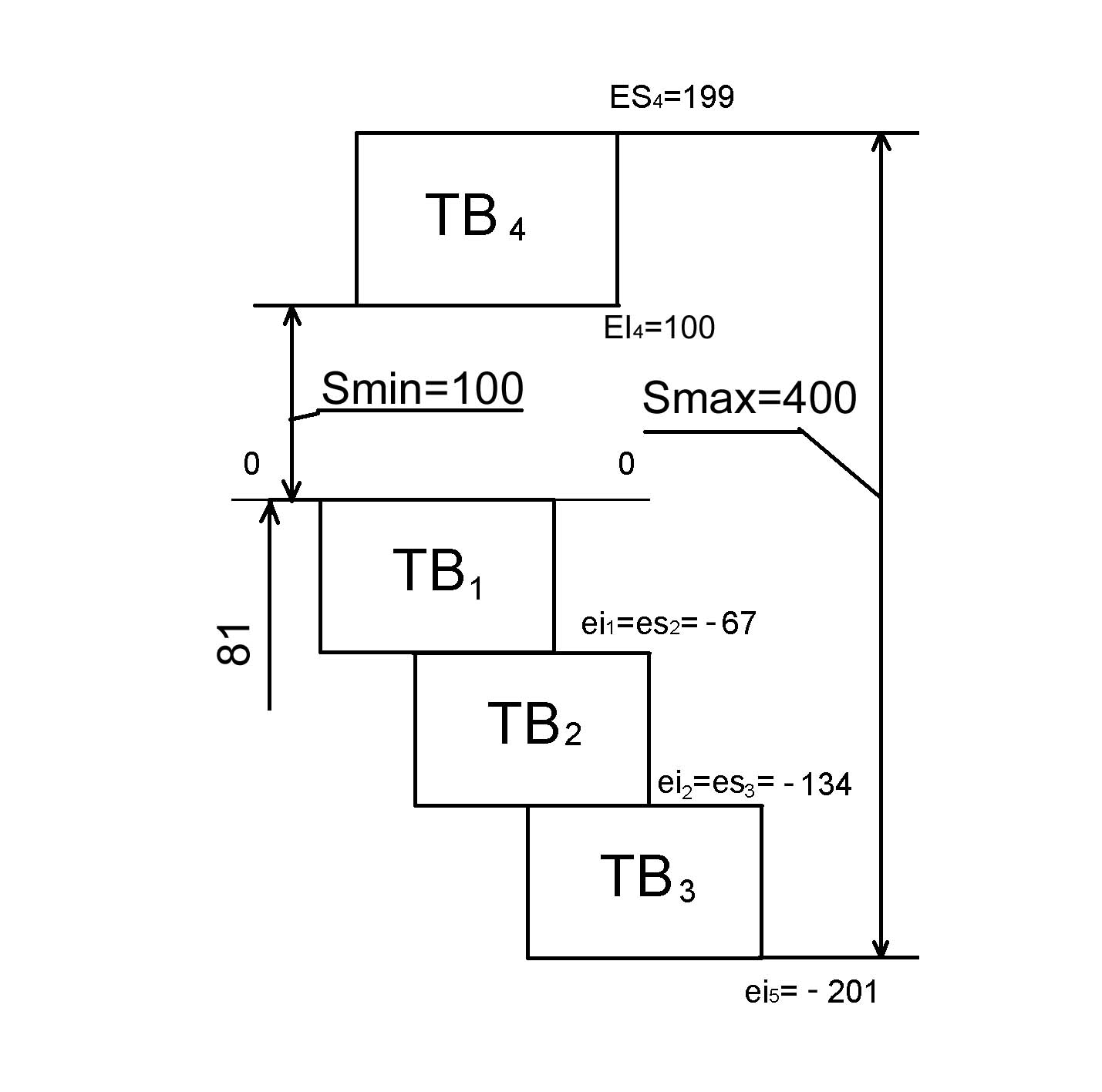
Let us present the details of unit 1 with nominal dimensions and tolerances, prepared for assembly. We will receive in the graphic chain, as it was, ordered: S max = 400 µm and S min = 100 µm.
Bushing Gear Bushing
Drawing. Component parts of the assembly with dimensional tolerances and their chain of location
The solution of the problem by the method of tolerances of one quality-complete intermeasurement (MPV).
Let's solve the same problem, but according to the dependencies of the method of complete interchangeability, without finding tolerances according to the dependence of the method of one quality. When determining the tolerance, for the dimensional chain "A" we will use the formula to calculate the tolerance through the accuracy factor "a":
It is necessary to determine a and i:
Assuming that the manufacturing accuracy of all parts of the same level, we can assume that all accuracy coefficients are the same equal to a Wed ... This coefficient can be obtained:
If there are parts with specified tolerances, then the formula takes the form:
Finished parts tolerances, such as those obtained through cooperation. We have no given tolerances, so the second sum in the numerator is zero. The closing dimension tolerance will be:
Now the dimensional tolerances will be:
which corresponds to the result previously obtained by the equal tolerance method.
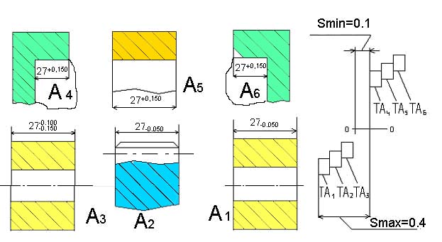
In the general case, the method of tolerances of one quality assumes the presence of different sizes of links. For the previously considered problem, we will assume that the body is one-piece and its internal size is 81 mm.
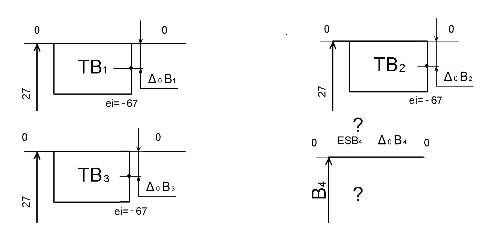
For node 2, select the dimensional chain and designate it as "B":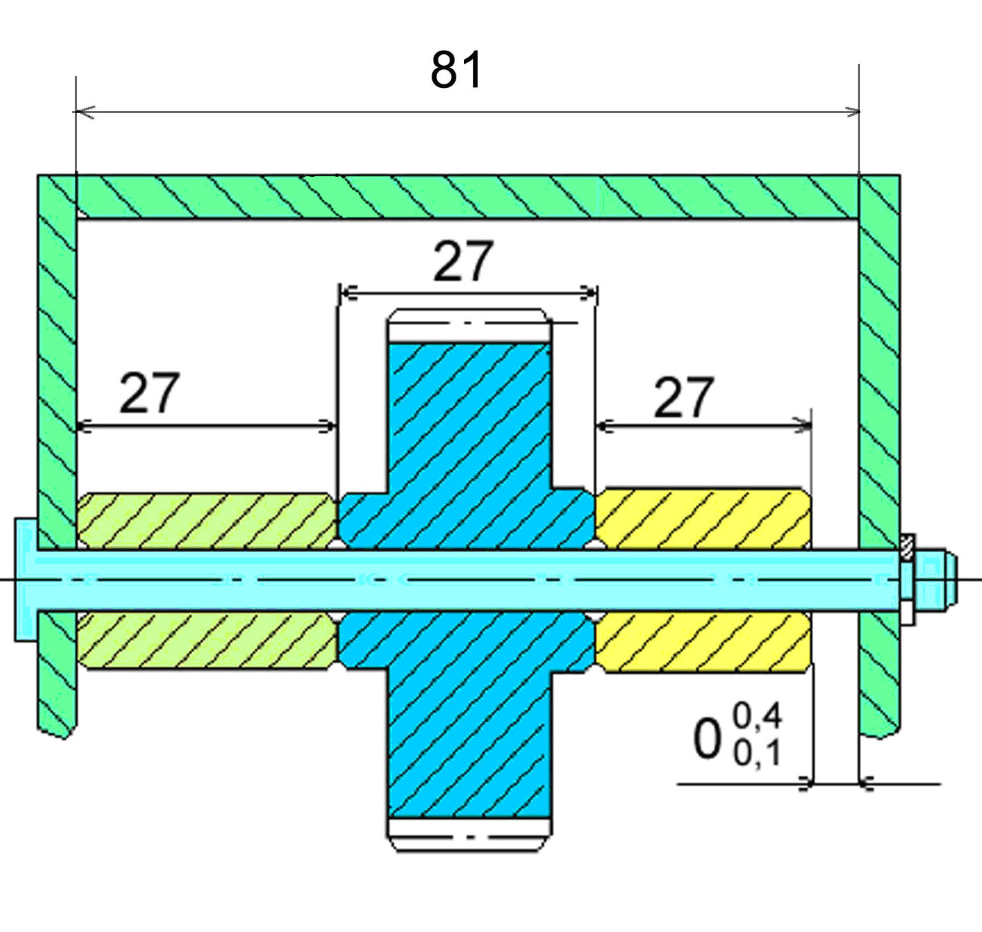
Drawing. Node 2.
The dimension chain will now look like this:
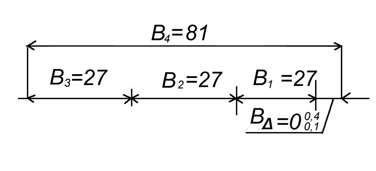
Drawing. RC-V
There are no dimensions with specified tolerances, therefore:
Let's check the sum of the tolerances:
67,07+67,07+67,07+98,781=201,444+98,549=299,871
Rounding up the tolerances to 67 and 99 microns, we get:
67+67+67+99=300
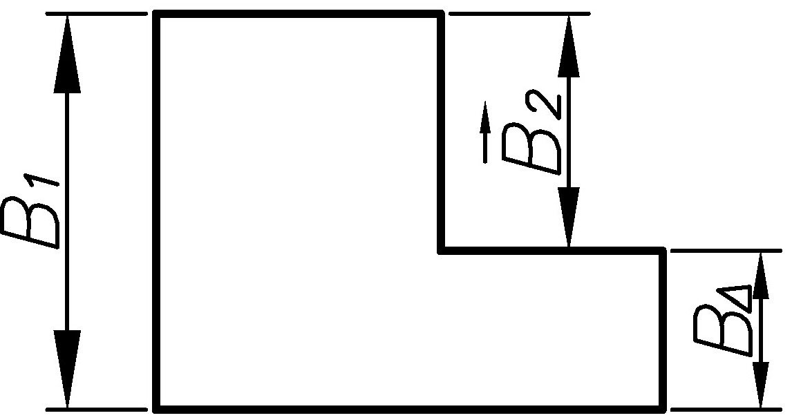
Accept dimensional tolerances B 1, B 2, B 3 into the body of admission, and B 4 as the linking size:
Drawing. Fields-B
Using the equation for the maximum value of the closing size, we get:
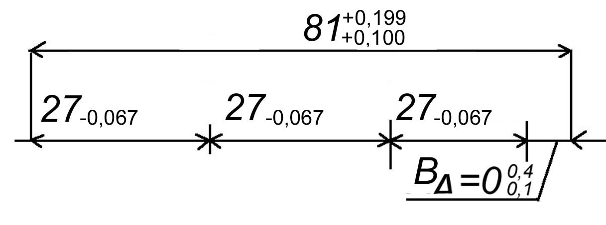
Drawing. RC-V with dimensional deviations
Now, having presented the obtained result graphically and check the obtained values of the closing size:
Drawing. Graphic chain of tolerance fields B
Equations can also be checked:
Based on the results of solving the equations and graphically, you can see that the problem has been solved, right.
However, let us carry out an additional check by means of the equation of the middle of the tolerance fields:
Here it is indicated 0 - the middle of the tolerance range of the corresponding size.
Let us find the midpoints of the fields of known tolerances, with the exception of the linking tolerance, and denote the values in the figure:
The location of the tolerances is the same, therefore:
Determine the middle of the tolerance field of the closing size:
Substituting the values into the equation, we find the middle of the tolerance field of the linking size:
By graphical check also:
Determine the deviations of the linking size:
Determine the average size of the gap, through the tolerances along the graphic chain: (100 + 199) / 2 + (0 + 201) / 2 = 149.5 + 100.5 = 250μm
The solution of the problem by the probabilistic-theoretical method (TVM).
For node 2, select the dimensional chain and designate it "C":

Drawing. RC-S
The problem can be solved according to the probabilistic-theoretical method, for which the connection of the closing size with the component will be:
Accuracy coefficient "a" will take the form:
The quality is already greater than in the MPV, and you can calculate the tolerances and represent the position of the fields, for all sizes, except for the link:
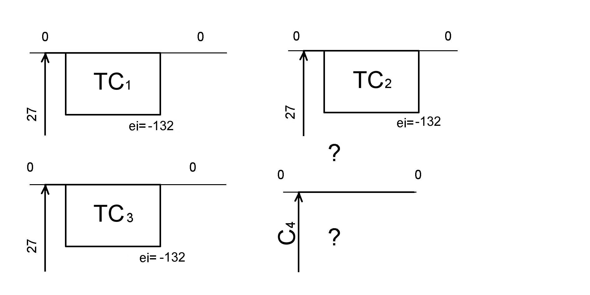
Drawing. Fields C
Let's use the equation:
and define the tolerance of the linking size:
,
We determine the midpoints of the tolerance fields of the constituent links of the RC and the closing size in order to use the equation:
We write the equation of the midpoints of the tolerance fields in terms of size tolerances:
The value of the average probable gap will be:
The final dimensional chain will be:
Drawing. Final dimension chain "C"
As you can see, the average size of the gap of 250 microns remained the same as in the solution by the method of complete interchangeability (MPV), but the tolerances have grown significantly.
The obtained results of the calculation by the probabilistic-theoretical method (TVM) can be represented graphically:

Drawing. CHAIN C
After evaluating the tolerance ratios, we obtain the tolerance expansion coefficient for TVM in relation to MPV: K 1 = K 2 = K 3 = 132/67 = 1.97 K 4 = 193/99 = 1.94 K cf = (1.97 + 1.94) / 2 = 1.95. Now, it is enough to recall the curve of dependence of tolerance T and cost of parts C to notice that the cost of production will not fall by 2 times, but significantly more with the probability of a unit not being assembled at the level of 0.27% (only 3 assemblies per 1000 will not be assembled). And of course there is no doubt that the loss of 3 builds has already paid off.
Drawing. Correlation between the size of tolerances and cost
Solving the problem by the compensation method
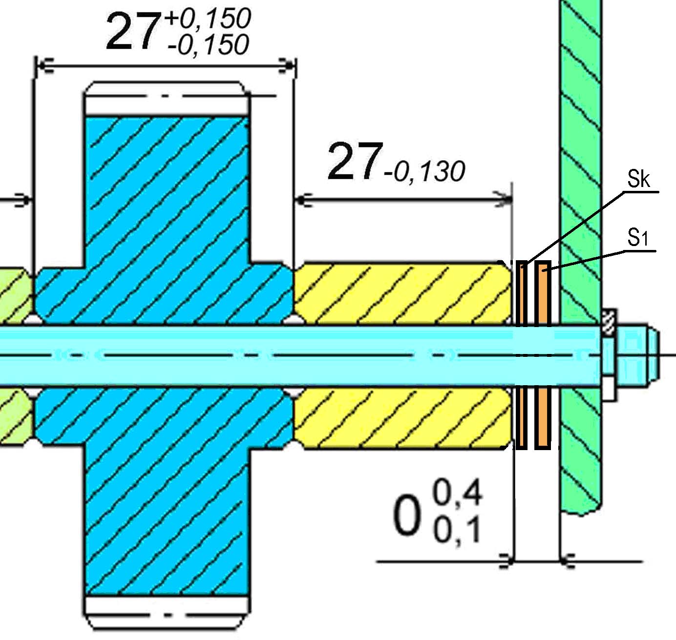
Drawing. ASSEMBLY 3L
Let's call the dimensional chain " L "

Drawing. CHAIN L1
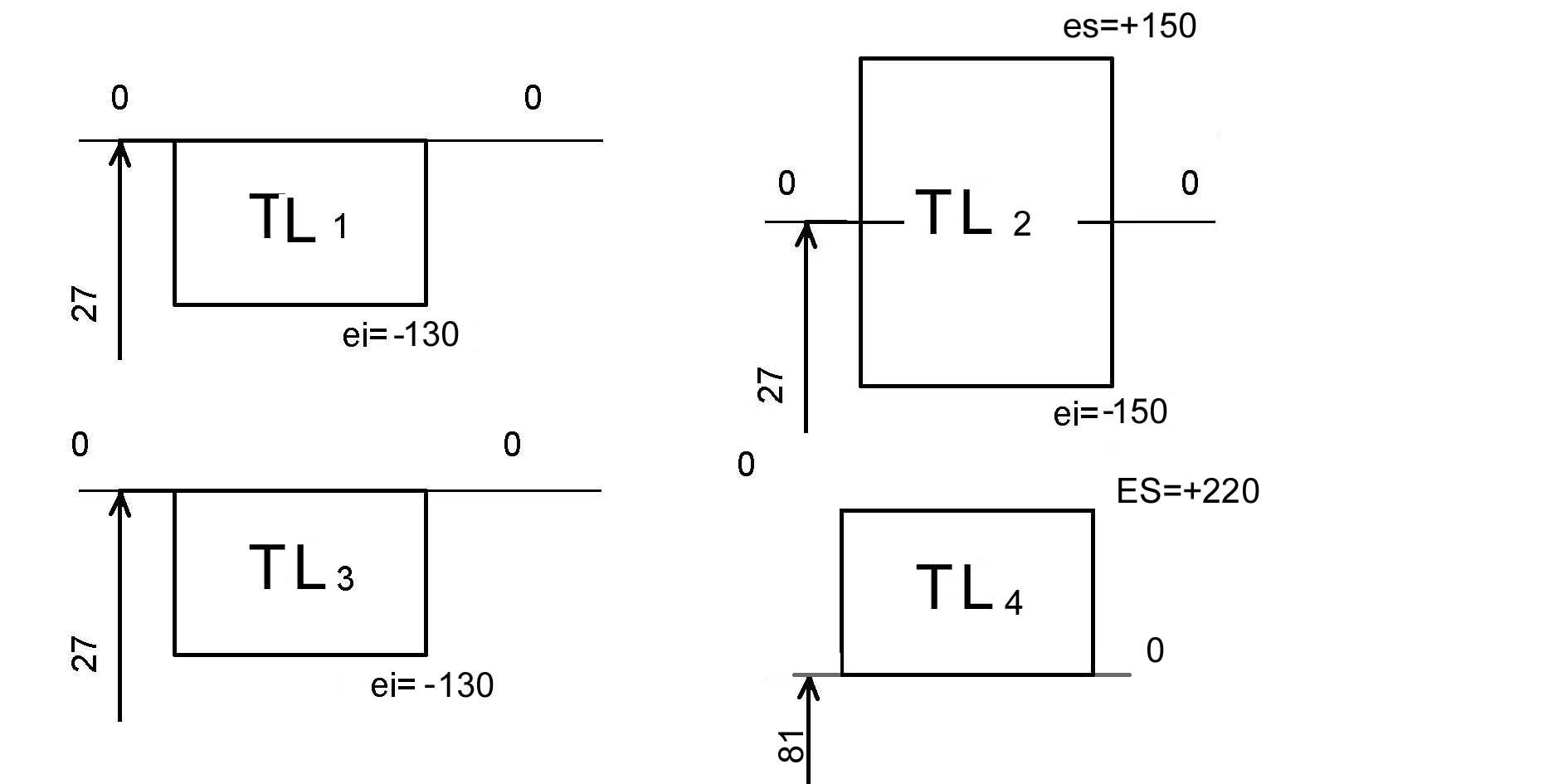
If one of the dimensions already has deviations, set the dimension L 2 preset = 27 0.150, then the size tolerance will be 0.3, but the closing tolerance is also 0.3. Substituting the values into the dependence for the accuracy coefficient, we obtain the uncertainty.
The resulting 0 in the numerator does not allow solving the problem ... ..
Accept part body tolerances for L 1, L 3, L 4 by grade 11 and determine their values according to the tables of standards:
TL 1 = TL 3 = 130 TL 4 = 220
Drawing. CHAIN L1 with dimensional deviations
Notice, that:
L 1, L 3 - the covered dimensions, therefore, assigning a tolerance to the body of the part, we get 27-0,130
L 4 - spanning size, therefore 81+0,220
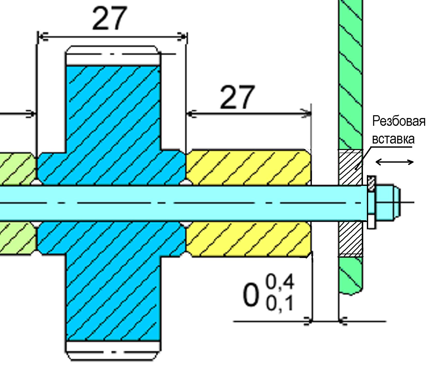
Drawing. Assembly with a movable expansion joint
To ensure smooth compensation, it is necessary to prepare a connection with a low axial feed (for example, with a thread with a pitch of P = 0.5 mm, the compensation limit will be selected ~ per 1 revolution). To ensure the required closing dimension, it is necessary to tighten the compensating plug until the gap is closed, and then unscrew 1/2 turn, which will provide a closing dimension of 250 μm, which is the middle of the closing dimension tolerance field. Next, it is necessary to prepare a threaded hole in the recess of the fixing nut and fix it with an M4 screw. Otherwise, vibrations can loosen the connection and disrupt the alignment.
As you can see, although such a solution is convenient, it technologically requires a special unit, cumbersome, albeit easy to adjust. In structures, it is often more convenient to use rigid expansion joints, the number of which can be calculated.
By MPV?
You can't decide.
Similarly to TBM, L 1 L 2 L 3 is assigned according to IT 11,
TA 1 = TA 3 = 130
TA 4 = 220
Drawing. FIELDS L
but ТLΔ d.b. is equal to ТL i
Let's check:
300 130 + 300 + 130 + 220.300 780
to satisfy equality, we introduce a compensator and write
Т L Δ = L А i - ТL к ТL к = ТL i - ТLΔ
TL k = 780 -300 = 480
(81.0 + 0.220) - ((27.0 - 0.130) + (27.0 - 0.150) + (27.0 - 0.130)) - 0.400
81.220 - (26.830 + 26.850 + 26.870) - 0.400
0.230
81 - (27 + 27.150 + 27) - 0.1
81 - (81.150 + 100)
0.250 negative complex?
![]()
Drawing. Compensation field 1
So, in one case, add gaskets, in the other - remove 250 microns
The resulting version solves the problem only partially, since -0.250 will have to be cut ..., and +230 leads to going beyond L .
Reduce the size L 1 by 1 mm, and now. L 1 = 26mm.
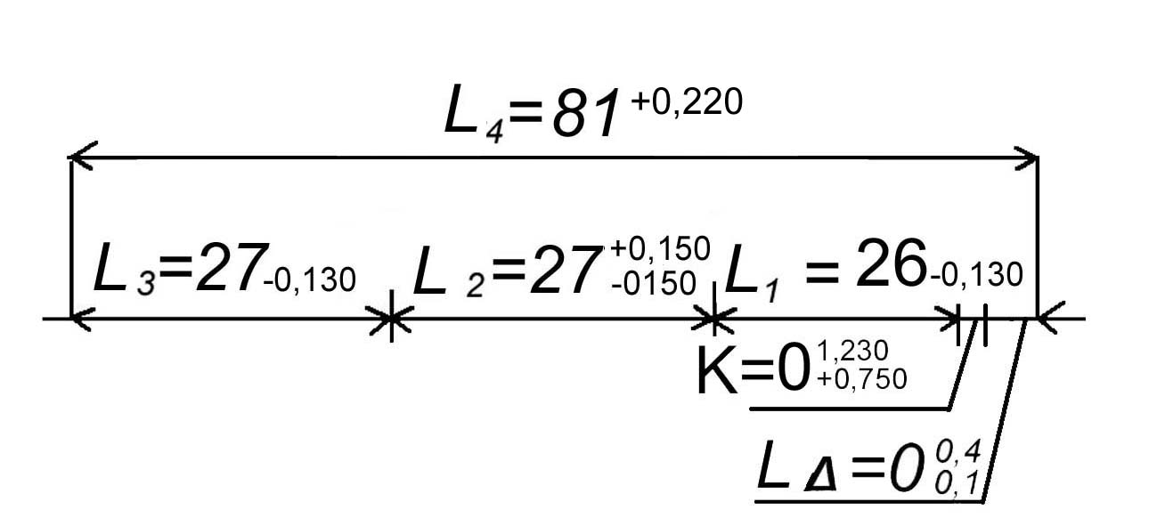
Drawing. Final chain L
Then:
81.220 - (26.830 + 26.850 + 25.870) - 0.400
81.220 - 79.990 = 1.23 mm
81 - (27 + 27.150 + 26) - 0.1
0.750
T L k = 1.23 - 0.750 = 0.480 mm
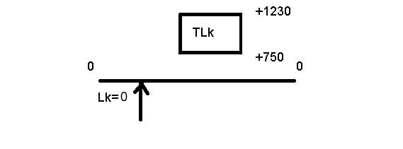
Drawing. Compensation field 2
The thickness of the first permanent spacer corresponds to the minimum compensation S 1 = 0.750mm.
Number of compensation steps
if necessary, it should be rounded up.
Now we will determine the thickness of the expansion gaskets, if their number is known and when they are applied, they must fit within the limits of the closing size:
there is for R 20, but it is better for R 10 to take S = 0.25mm,
then N
rounded up is 2.
It is now clear that the expansion joint consists of one permanent 0.750mm spacer and two replaceable 0.250mm spacers.
Upon compensation, we will receive the dimensions:
Let's check the compliance with the inequality:
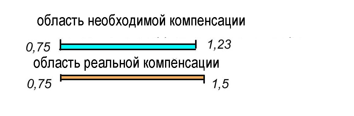
Drawing. Compensation area
Conclusion :
As you can see, the largest tolerances of the component links are in the compensator method (MC). It is followed by the probability-theoretic method (TVM). The tightest tolerances in the full interchangeability method (FIF). This method is good, but too expensive. The compensator method requires adjusting the introduction of additional parts and even assemblies, but wide tolerances in mass production compensate for all costs, in other cases it is rational to use MPV and TVM.
Other similar works that may interest you. Wshm> |
|||
| 3864. | Microwave. Microwave electronic circuits | 901.27 KB | |
| Typical examples of volume-distributed circuits are waveguides, resonators and similar elements of microwave technology. The class of linearly distributed circuits includes two-wire and coaxial lines ... | |||
| 1849. | Analysis of the electrical circuit of the control system | 242.12 KB | |
| Task option number Figure number Electrical circuit parameters Analyze the electrical circuit of the control system. Designate circuit nodes and branch currents; indicate input and output signals; Determine the transfer function of the two-port network; Determine and present graphically the amplitude-frequency response and phase-frequency response characteristics; Using the obtained differential equation, construct a structural diagram ... | |||
| 3876. | OHM'S AND KIRCHHOF'S LAWS. POTENTIAL CIRCUIT DIAGRAM | 14.47 KB | |
| Summary work In the process of performing work, measure: the voltage current on the elements in an unbranched circuit and check Ohm's law; the strength of the voltage current on the elements in a complex circuit and check the Kirchhoff's laws; check the principles of superposition for a linear circuit. The potentials in the circuit are determined analytically and compared with experimental data. Preparation for work How the first and second Kirchhoff laws are formulated Why, when calculating a circuit, the number of independent equations compiled according to ... | |||
| 9446. | Input circuits of radio receivers of various ranges | 2.52 MB | |
| Taking into account these remarks, the input circuit can be defined as a part of the high-frequency channel of the HFT intended for the coordinated transmission of signals from the antenna to the input of subsequent stages and suppression of side reception channels, with the exception of the adjacent channel .; low noise figure; constancy of parameters over the range; little effect of changing the antenna on the operation of the radio receiver. For symmetrical vibrators, the geometric length of which is much less than a quarter of the wavelength, the following relations are true: antenna impedance resistance ... | |||
| 5552. | Application of the MathCad system for studying a linear electric circuit of sinusoidal current | 308.97 KB | |
| The purpose of this course work is to use the MthCd system to study a linear electrical circuit of sinusoidal current. The paper investigates the influence of the frequency of the supply voltage on the amplitude of the input current of the electric circuit. The objectives of the course work: combining all previously acquired knowledge in the MthCd system and applying them in practice, consolidating the theoretical knowledge of the MthCd package for the analysis and calculation of AC electric circuits ... | |||
| 1694. | 1.44 MB | ||
| It contains a converting device (CRD), defined as an electrical device that converts the type of current, voltage, frequency and changes the quality indicators of electrical energy, designed to create a control action on the electric motor device. | |||
Sixth lecture
5. Dimensional chains
Plan
General information about dimensional chains.
Types of dimensional chains
Tasks of calculating dimensional chains
Numerical example of the design calculation of the dimensional chain
Interchangeability is determined not only by the accuracy of pairwise connections, but often by the total accuracy of a complex of structural elements (machine, device).
Dimensional chain (RC) - a set of dimensions related to the product, directly involved in solving the problem (design, technological, measuring) and forming a closed loop (chain). Each size is a link in such a chain.
In any DC there is always one link, called the closing link, which is physically obtained last (during manufacture, assembly or measurement). When the problem of calculating the RC is formulated, this link is the initial one.
Rice. 5.1. Measuring dimensional chain diagram
So, for the case of measuring the size A Δ shown in Fig. 5.1 parts, this size is the closing link, since it can be determined only after measuring other dimensions of the chain formed here - a closed loop of dimensions A1 - A Δ - A 3 - A 2 - A 1.
A diagram of the structure illustrating the assembly DC is shown in Fig. 5.2. The basis of this design is the housing 1. It has two centering units (2 and 2 "), which provide a centered position relative to them of the sensitive element 3 of the inertial device (the system for maintaining its position coaxial with the nodes 2 and 2" is not considered). The closing link in the corresponding dimensional chain (Fig. 5.3) is the total clearance (А Δ "+ А Δ" ").
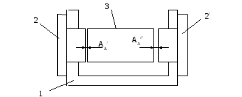
Rice. 5.2. Diagram of the layout of the system of axial magnetic centering of the float sensitive element: 1 - body; 2, 2 / - centering nodes; 3 - centered element.
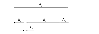
Rice. 5.3. Diagram of the dimensional chain of the structure of the layout of the axial centering system
The rest of the RC sizes - constituents... All of them in relation to the closing (initial) link are divided into augmenting and reducing dimensions (links), depending on whether the closing size increases or decreases with an increase in the considered component link.
The most elementary special case of RC is the connection of the shaft and the hole (consider for a positive clearance):
Rice. 1.5.4. Representation of landing as a special case of RC: A 1 - hole size, A 2 - shaft size, A 0 - clearance (closing link); a) structural diagrams; b) RC diagram
The dimensional chain (RC) is called linear if its links are linear dimensions. Dimensional chains, the links of which are angular dimensions, are called angular dimension chains... A dimensional chain is called flat if all its links lie in one or more parallel planes. A dimensional chain is called spatial, all or part of the links of which are located in non-parallel planes.
The simplest are one-dimensional (collinear) linear RC (Fig. 5.1, 5.3, 5.4, b). If the RC links are not parallel, then A j is taken as the projection of the corresponding vector onto the line of the closing size.
Tasks of calculating dimensional chains
The operational properties of machines, devices and many other products depend mainly on the closing link of the RC. It is for the closing link during the development of the structure that the interval (A Δe, nm, A Δe, nb) of operational permissible values should be established. The accuracy of the constituent links of the RC plays a subordinate role: the intervals of permissible values of these dimensions should be established based on a given interval (A Δe, nm, A Δe, nb). Quite reasonably, the closing link is also referred to as the original one.
The main task solved at the design stage (task of the design calculation of the RC): determine the intervals of permissible values of the dimensions of the constituent links for a given interval (A Δe, nm, A Δe, nb) of the operationally permissible values of the closing link. This problem (also called the synthesis problem) can be formulated in relation to the limiting deviations.
If the maximum deviations of the constituent dimensions are known (as a result of solving the design problem), then to check their compliance with the interval (A Δe, nm, A Δe, nb), the inverse problem is solved.
Design ratios required to solve RC problems
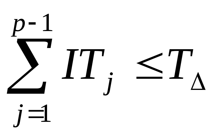
The starting ratio connecting parallel links:
 , (5.1)
where m is the number of increasing sizes; p is the total number of links (together with the original).
Expressions for the largest and smallest values of A Δ follow from (5.1):
 ; (5.2)
 . (5.3)
Hence, based on the definition of the tolerance T of size A as
T = A nb - A nm (5.4)
it is easy to get a formula linking the tolerances of all links:
 . (5.5)
That is, the tolerance of the closing link is equal to the sum of the tolerances of the constituent links, which has a completely obvious meaning: it is impossible to obtain a high total accuracy of manufacturing, assembly, measurements without a correspondingly high accuracy of the elements that make up the result of these processes.
To solve the problems of the RC, it is also necessary to have ratios connecting the limiting deviations of the links. They can also be deduced from the starting expressions (5.2), (5.3), taking into account that
A j nb = A j + E s (A j); A j nm = A j + E i (A j), (5.6)
where E S, E i - upper and lower limit deviations.
 ; (5.7)
 . (5.8)
Now you can solve the problems of calculating the RC. It should be emphasized that the formulas obtained above are used to solve problems subject to complete interchangeability (maximum-minimum method).
Methods for solving the problem of design calculation of the RC
Here it is necessary, firstly, to distribute the tolerance of the closing link among the constituent links, and, secondly, to assign maximum deviations. The first part of the task can be accomplished in two ways:
Equal tolerances;
Equal tolerances.
Simpler, but at the same time, rude - equal tolerance method:
T j = T cf = T Δ / (p-1),  (5.9)
(5.9)
The resulting value should be rounded to the standard (s), and then check the condition
 .
.  . (5.10)
This method gives good results only for RCs with similar component links. If the constituent dimensions of the chain differ significantly in size, then the qualifications of their accuracy will also differ greatly. For example, IT = 25 μm tolerance corresponds to grade 9 for size 3 mm and grade 5 for size 400 mm. Such a difference in the quality of accuracy is uneconomical (after all, as already noted, each more accurate quality is given at a non-linearly increasing cost).
When solving the problem by the method equal tolerances strive to get the tolerances of the constituent dimensions for the same quality. Therefore, the tolerance of each link must contain the same number n of tolerance units.
Thus, here they proceed from the formula
IT j = n cf * i j (A), (5.11)
where i j (A) is the tolerance unit of size A.
Hence, the required number of tolerance units is found as
 . (5.12)
The obtained value of n cf makes it possible to choose the number of qualifications so that the condition (5.10) is fulfilled.
After the tolerances are assigned, it remains to find the maximum deviations. It is most convenient to do this, following the well-known rule: the tolerance field of each of the sizes of the enclosing internal elements is considered the tolerance field of the main hole (Figure 5.5, a), the tolerance field of each of the dimensions of the covered external elements is the tolerance field of the main shaft (Figure 5.5, b) , and the tolerance fields of the links that do not belong to the shafts or to the holes are considered symmetrical with respect to the line of the nominal size (Figure 5.5, c). This rule should be applied to all constituent dimensions, with the exception of one - linkage or reserve. Two limiting deviations of this reserve link remain unknown, determined from two equations.
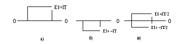
Rice. 5.5. To the choice of maximum deviations of the constituent links of the dimensional chain (design calculation)
Given. Dimensional chain (Fig.5.3) related to the structure shown in Fig. 1.5.2. The size of the magnetic gap А Δ is set in the following operating range: 40 ≤ А Δ ≤ 150 μm. Nominal dimensions:
A 1 = A3 = 10 mm; A 2 = 80 mm; A 4 = 60 mm.
It is required to determine the maximum deviations E i (A j) -?, E s (A j) -?
Solution. The number of tolerance units n cp is calculated by the formula (5.12) with the following values of tolerance units i j:
i 1 = i 3 = 0.9 μm; i 2 = i 4 = 1.9 μm.
n cp = 110 / 5.6 = 19.6.
The resulting number gives grounds to take tolerances for qualifications 7 and 8. Let IT 1 = IT 3 = 22 microns (8th quarter); IT 2 = IT 4 = 30 μm (7th sq.)
Σ IT j = 104 μm, which is about 6% less than the width of the specified operational interval.
Now it is necessary to determine the boundaries of the tolerance fields E i (A j) -?, E s (A j) -?
We assign A 2 (the distance between the end surfaces of the body) as the linking (backup) link. For size A 4, we take the tolerance field of the main shaft (Fig.5.5), and for dimensions A 1, A 3 - tolerance fields symmetrical about the line of the nominal size.
Equations (5.7), (5.8) in the considered case have the form:
E S Δ = E S2 - E i1 - E i3 - E i4;
E i Δ = E i2 - E S1 - E S3 - E S4.
The unknowns E S2 and E i2 are determined from these equations:
E s2 = 150 - 22 - 30 = 98 microns; E i2 = 40 + 22 + 0 = 62 microns.
Tolerance T = 36 microns is rounded to the standard IT = 30 microns.
Literature
Belkin V.M. Tolerances and fits (Basic standards of interchangeability). - M .: Mechanical Engineering, 1992. - 528 p.
Dunin-Barkovsky I.V. Interchangeability, standardization and technical measurements. - M .: Publishing house of standards, 1987 .-- 352 p.
A.I. Yakushev Interchangeability, standardization and technical measurements. - M .: Mechanical Engineering, 1986.
A machine or mechanism assembled from individual parts will work normally only if each part is made with a given accuracy and correctly occupies its intended place among other parts, performing its functions. The required position of the surfaces of the parts and their axes relative to other parts in the assembled product is provided by the calculation of dimensional chains.
Dimension chain is a set of interconnected dimensions that form a closed loop and are directly involved in solving the problem. Dimensional chains can be: design, technological, measuring. The design dimensional chain is drawn up to solve the problem of ensuring accuracy in the design of the product, the technological one - to solve the problem of ensuring accuracy during manufacture, and the measuring chain when measuring the quantities characterizing the accuracy of the product.
The basis for drawing up and calculating linear and angular dimensional chains is RD 50-635-87.
All sizes included in the dimensional chain are called links and are designated by one capital letter of the Russian alphabet with the corresponding index. The links of the dimensional chain are divided into components and closing. There can be only one closing link. This is the link that is obtained last as a result of solving the problem in the manufacture of a part or assembly of an assembly unit, as well as during measurement. There can be a different number of constituent links, determined by the purpose of the product and the solution to the problem.
Figure 9.1 shows examples of the simplest three-link dimensional chains, where A 1 and A 2 are the constituent links; And Δ is the closing link.
The constituent links affect the closing link in different ways. Depending on this influence, they are divided into increasing and decreasing.
Increasing such links are called, with an increase in the size of which the closing link increases, and reducing those, with an increase in which the closing link decreases.
In Figure 9.1, link A 1 - increasing, A 2 - decreasing. In more complex dimensional chains, it is convenient to use the closed loop traversal rule. For this purpose, the closing link is given an arbitrary direction with an arrow placed above the link designation (Figure 9.2) and bypasses all links, starting with the closing link so that a closed flow of directions is formed. Then all the links that have the direction of the arrows on the dimensional chain diagram the same as the closing one will be decreasing, and all the others will be increasing.
If the direction of the closing link is always set only to the left, then when walking along a closed contour, all component links with the direction of the arrows to the left will decrease, and with the direction of the arrows to the right, they will increase. This particular case of the general closed-loop traversal rule is often used.
Depending on the relative position of the links, dimensional chains are divided into linear (with parallel links), flat and spatial. All dimensional chains are calculated using the formulas for linear chains. Spatial dimensional chains lead to flat, and flat to linear ones by projecting the dimensions of the chain in one direction, which is usually the direction of the closing link.
The calculation of dimensional chains is a mandatory step in the design of machines. It helps to ensure interchangeability, improve product quality and reduce manufacturing labor intensity. The calculation of dimensional chains consists in finding the tolerances and maximum deviations of all chain links based on the requirements of the design and manufacturing technology.

When solving dimensional chains, two tasks are distinguished:
It is necessary to determine the nominal size, tolerance and maximum deviations of the closing link according to the known nominal dimensions and maximum deviations of the leaving links. This problem is called inverse and is often used for verification calculations. It has an unambiguous and fairly simple solution.
It is necessary to determine the tolerance and maximum deviations of all component links according to the known nominal dimensions of the links, the tolerance and maximum deviations of the closing link. This problem is called direct. It is quite complex and has several solutions.
Dimensional chains can be solved by methods that give different results. So, RD 50-635-87 provides for the following methods: full interchangeability (maximum - minimum); incomplete interchangeability (using the provisions of the theory of probability); group interchangeability; fit method; regulation method.
Accepted designations:
A 1 A 2; ... A j - designation and nominal size of links of the dimensional chain A;
A Δ - designation and nominal size of the closing link of the dimensional chain A;
A j - increasing j-e component link of the dimensional chain A;
A j - decreasing j-e component link of the dimensional chain A;
Compensating j-e component link of the dimensional chain A;
n is the number of increasing links;
p is the number of decreasing links;
m - 1 - the total number of constituent links: n + p = m - 1;
m is the number of links in the dimensional chain;
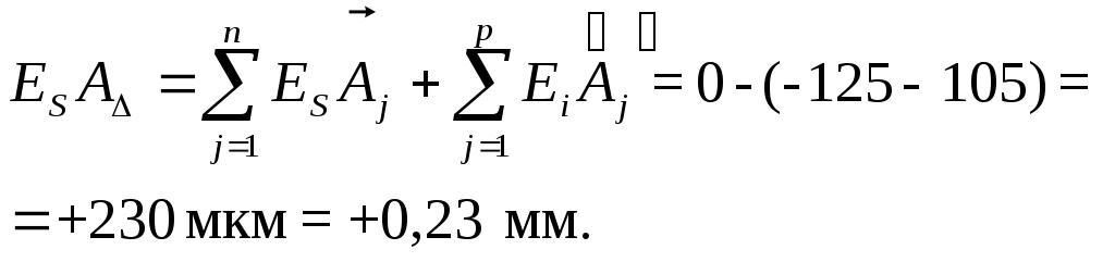
E S A Δ - upper limit deviation of the closing link of the dimensional chain A;
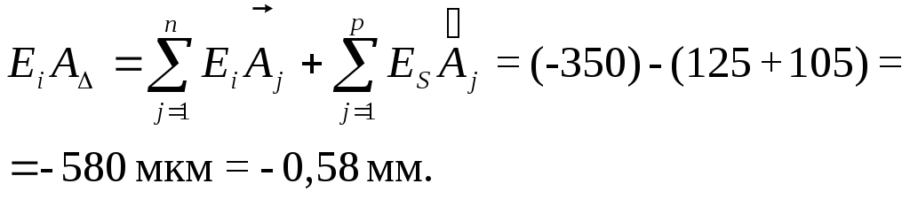
E i A Δ is the lower limit deviation of the closing link of the dimensional chain A;
E S A j- the upper limit deviation of the component link of the dimensional chain A;
E i A j- the lower limit deviation of the component link of the dimensional chain A;
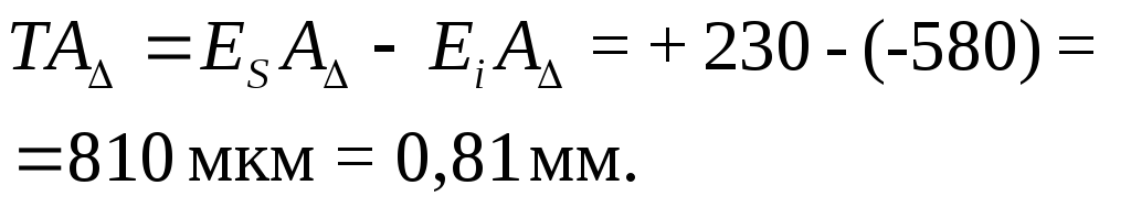
TA Δ - tolerance of the closing link of the dimensional chain A;
TA j- tolerance of the j-ro link of the dimensional chain A;
E with A Δ - coordinate of the middle of the tolerance field of the closing link of the dimensional chain A;
E c A j- coordinate of the middle of the tolerance field j-ro of the component link of the dimensional chain A;
E WITH V A Δ - coordinate of the middle of the scattering field of the closing link of the dimensional chain A;
E cv A j - coordinate of the middle of the scattering field j-ro of the component link of the dimensional chain A;
E m A Δ - coordinate of the center of grouping of the closing link of the dimensional chain A;
E m A j- coordinate of the center of grouping j-ro of the component link of the dimensional chain A;
V k is the amount of compensation;
λ is the relative standard deviation;
t Δ - risk coefficient;
α is the coefficient of relative asymmetry;
ξ A j- gear ratio j-ro of the link of the dimensional chain A;
N is the number of steps of the dimensions of the fixed compensator;
p is the percentage of risk.
Basic calculation formulas [ 33 ]
The nominal size of the closing link of the dimensional chain A is determined by the formula:
 , (9.1)
where j = 1,2, ... m is the serial number of the dimensional chain link; ξ A j- gear ratio j-ro of the link of the dimensional chain A.
Depending on the type of the dimensional chain, the gear ratio may have a different content and meaning. So, for example, for linear dimensional chains (chains with parallel links), the gear ratios are:
ξ j= 1 for increasing constituent links;
ξ j= -1 and for decreasing component links.
For this reason, for linear dimensional chains, dependence (9.1) is written in the form:
 , (9.2)
where n is the number of increasing links; p is the number of decreasing links.
Closing link tolerance TA Δ calculated for maximum - minimum:
 (9.3)
(9.3)
Coordinate of the middle of the tolerance field E with A Δ of the closing link of the dimensional chain A:
 , (9.4)
Limit deviations of the closing link A Δ:
 , (9.5)
 . (9.6)
It is possible to determine the maximum deviations of the closing link according to the dependencies:
 , (9.7)
 . (9.8)
Limit dimensions of the closing link:
 ; (9.9)
 . (9.10)
When calculating by the probabilistic method, the tolerance of the closing link:
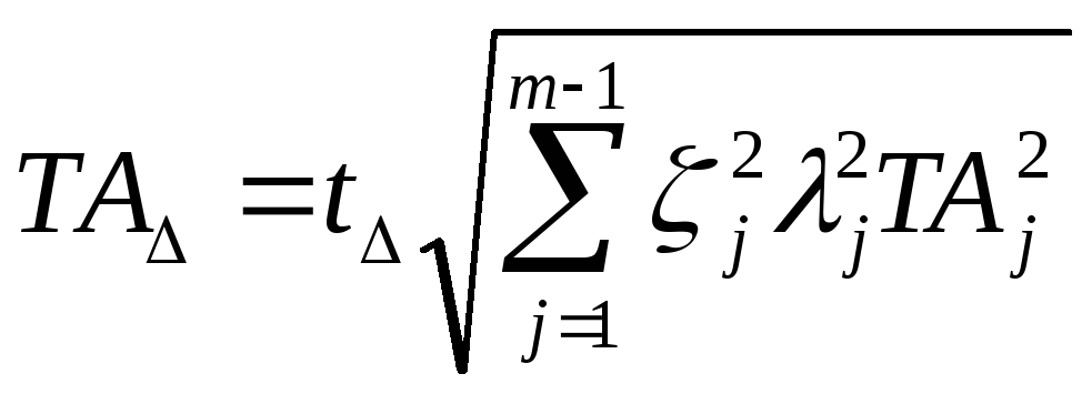 , (9.11)
where t ∆ is the risk coefficient taken from Table 9.1.
Table 9.1 - Risk ratio
|
Coefficient t ∆ |
For dimensional chains with parallel links (linear dimensional chains) ξ 2 j =1.
Coefficient λ 2 j= 1/9 with the normal law of distribution of deviations (Gauss's law).
With the distribution of deviations according to the triangle law (Simpson's law) λ 2 j = 1/6.
With the distribution of deviations according to the law of equal probability λ 2 j = 1/3.
Sometimes, in the calculations of dimensional chains, the coefficient of relative scattering K j= t ∆ λ j .
With the most frequently used risk percentage of 0.27, we have, according to Table 9.1, t ∆ = 3 and taking into account the values of the coefficient λ 2 j relative scattering coefficient K j is:
TO j= 1 with the Gaussian distribution law;
TO j= 1.22 with Simpson's law of distribution;
TO j= 1.73 with the law of distribution of equal probability.
When using the coefficient of relative scattering, equation 9.11 takes on a simpler form for linear dimensional chains with a percentage risk of 0.27
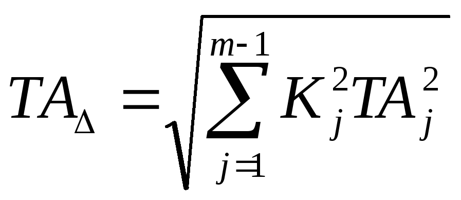 . (9.12)
The average value of the tolerance of the constituent links is calculated by the formulas:
when calculating according to the maximum - minimum method
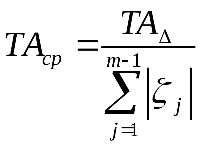 (11.13)
when calculating by probabilistic method
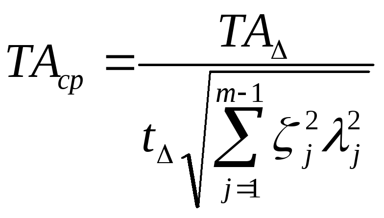 (11.14)
For linear dimensional chains, formulas (11.13) and (11.14) take on a simpler form when solved by the method of equal tolerances:
when calculating for maximum-minimum
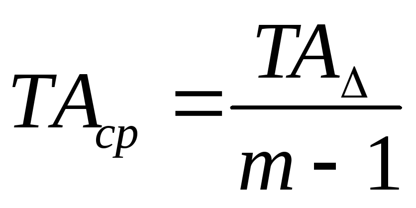 ; (9.15)
when calculating by probabilistic method
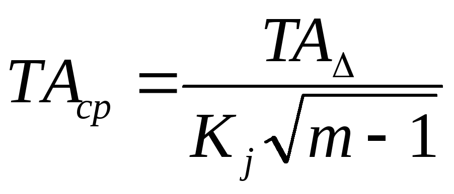 .
(9.16)
.
(9.16)
Solving the dimensional chain by the method of one quality, determine the number of tolerance units in the size tolerance (accuracy coefficient):
with full interchangeability (maximum-minimum)
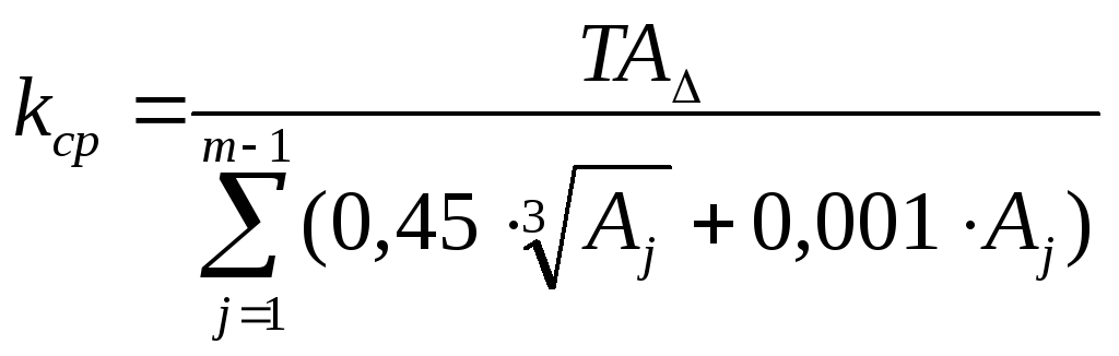 (9.17)
with incomplete interchangeability (probabilistic calculation)
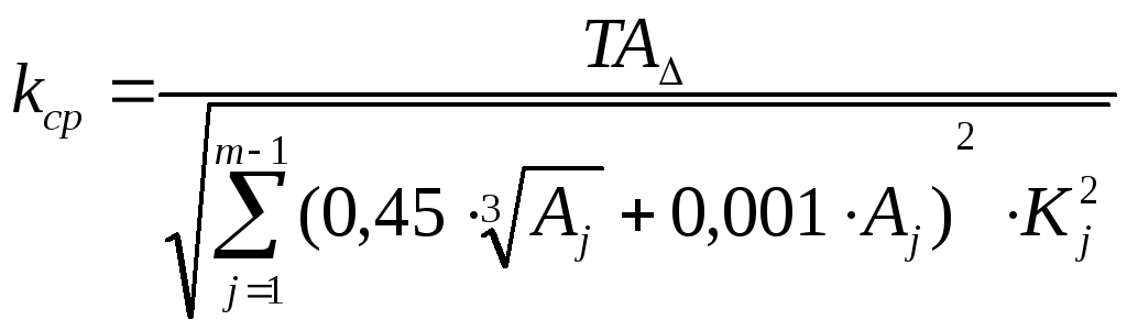 (9.18)
When solving the dimensional chain by the compensation method, the largest possible compensation V K is calculated:
V K = T "A ∆ -TA ∆, (11.19)
where T "A ∆ = ∑TA j- the manufacturing tolerance of the master link, equal to the sum of the extended tolerances of the links of the dimensional chain.
Number of stages of fixed expansion joints:
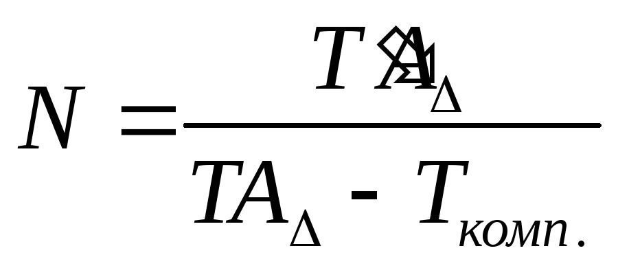 , (9.20)
where T comp. tolerance for the manufacture of a fixed expansion joint.
P
Figure 9.3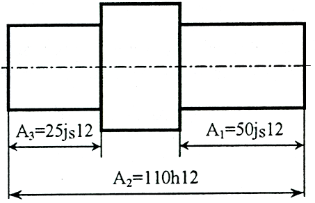
Draw up a dimensional chain and determine:
Closing link rated value;
Upper and lower deviation of the closing link;
Tolerance and limiting dimensions of the closing link.
Calculate in two ways:
a) at max - min; b) the probabilistic method with a risk of 0.27%, distribution of sizes according to the normal law with K j = 1; α j = 0.
Initial data: А 1 = 50js12; And 2 = 110h12; And 3 = 25jsl2.
Solution.
The problem is one of the converse ones and has an unambiguous solution. We draw up a dimensional chain diagram. The closing link of this dimensional chain is the axial dimension resulting from the latter as a result of manufacturing. This dimension is the axial dimension of the bead thickening. The dimensional chain diagram is shown in Figure 9.4.
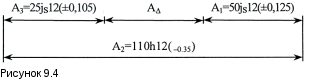
According to GOST 25346-89 (Tables A.2 - A.4), we find the values of the tolerances and deviations of the links and put them on the diagram: A 1 = 50jsl2 (± 0.125); And 2 = 110hl2 (-0.35); A 3 = 25jsl2 (± 0.105).
We identify the increasing and decreasing links of the dimensional chain. Let's set the direction of the closing link with the arrow to the left (Figure 9.5).
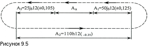
Using the rule of bypassing along a closed loop, we establish that links А 1 and А 3 are decreasing (the direction of the arrows bypassing along the contour coincides with the direction of the arrow of the closing link), and link А 2 is increasing.
Method "a" (calculation for max - min)
The nominal value of the closing link is found by the formula (9.2)
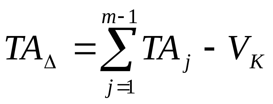
The tolerance of the closing link (formula 9.3), taking into account the fact that for linear dimensional chains | ξ j | = 1:
Upper deviation of the closing link (formula 9.7)
Lower deviation of the closing link (formula 9.8)
Examination:
Deviations are correctly identified.
The limiting dimensions of the closing link (formulas 9.9 and 9.10):
Master link size 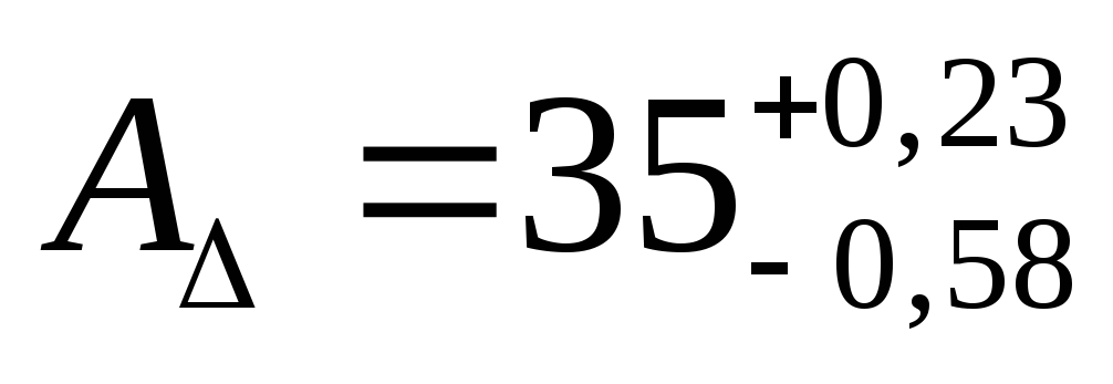 mm.
mm.
Method "b" (probabilistic calculation)
The nominal value of the closing link A ∆ is calculated by the formula (9.2) and was determined above A = 35 mm.
We find the tolerance of the closing link by the formula (9.12) taking into account the value of K j= 1 corresponding to the normal distribution
Let us find the coordinate of the middle of the tolerance field of the closing link (Equation 9.4), having previously determined the coordinates of the midpoints of the tolerance fields of the constituent links.
The diagrams of the tolerance fields of the dimensions that make up the chain are shown in Figure 9.6.
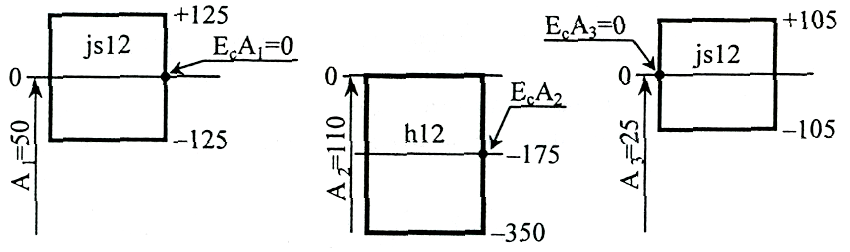
Figure 9.6
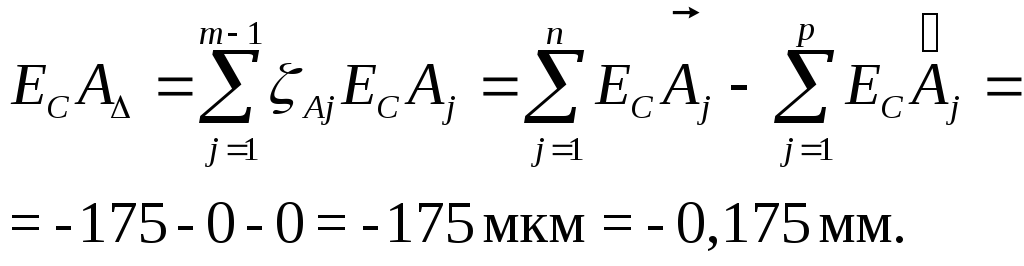
The upper deflection of the master link (equation 9.5):
Downward deflection of the mate (Equation 9.6):
The limiting dimensions of the closing link (equations 6.9 and 6.10)
Master link size 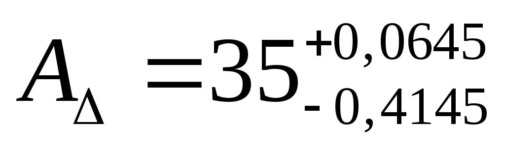 mm.
mm.
Calculation of dimensional chains by the regulation method
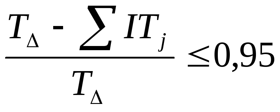
When calculating the dimensional chain by this method, the accuracy of the closing size of the dimensional chain is achieved by introducing a compensating link into the dimensional chain, which can be structurally made in the form of shims or in another way. All component links of the dimensional chain are assigned tolerances that are economically acceptable for the given production conditions (extended tolerances).
For such a dimensional chain, the condition must be met
 , (9.21)
where  - closing link tolerance
 - accepted extended tolerances of the constituent links
 - the amount of compensation
 . (9.22)
Compensating link nominal size:
 (9.23)
where  - the nominal size of the closing (initial) link;
 - the nominal dimensions of the increasing links;
 - the nominal dimensions of the reducing links;
Compensator nominal size;
n is the number of increasing links;
p is the number of decreasing links.
The "+" sign in front is taken when the increasing link and the "-" sign when the decreasing link.
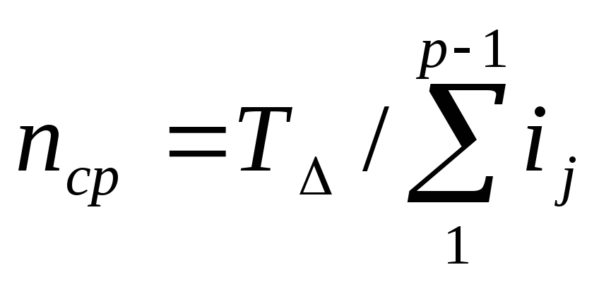
Required number of control steps:
 . (9.24)
The resulting n is rounded to the nearest whole number.
Smallest thickness of interchangeable gaskets:
 . (9.25)
The S value is rounded to the nearest smaller standard size in accordance with GOST 503-81 (cold-rolled steel strip made of low-carbon steel).
Number of replaceable pads
 (9.26)
The number of replacement shims can be reduced by using shims of different thicknesses. In this case, the thickness of each subsequent strip is taken:
 etc.
etc.
The final number of replaceable spacers is set when assembling the assembly unit, depending on the difference between the obtained value of the closing (original) link and the required value of this link.
Example... The fixing support of the gearbox shaft 1 consists of two tapered roller bearings 2; 3, placed in glass 4 (Figure 9.7).
Tightening of the inner rings of rolling bearings on the shaft in the axial direction is carried out through the spacer ring 5 with a nut 6 located at the threaded end of the shaft 1. The nut was locked against loosening by a lock washer 7 according to GOST 11872-89.
D
Figure 9.7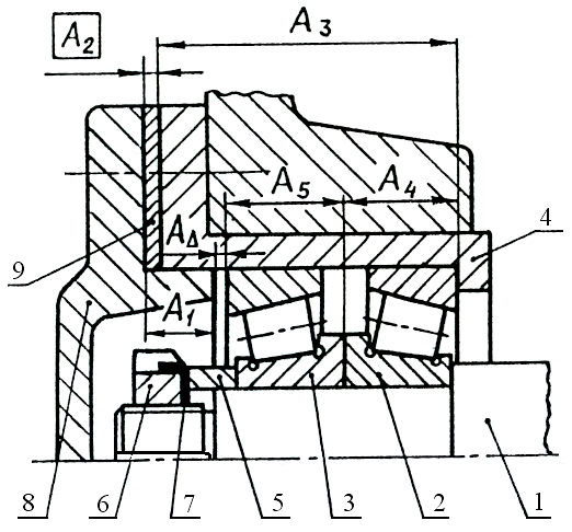
For bearing 7210, the inner ring diameter is d = 50 mm, the outer ring is D = 90 mm; mounting height T = 21.75 mm, permissible limits of axial play from 50 µm to 100 µm (table 8.4), maximum deviations of the mounting height of a rolling bearing of increased accuracy: top +0.2 mm; lower 0 (table A.25).
Draw up a dimensional chain and determine:
Nominal and limiting dimensions of the compensating link;
Number and thickness of interchangeable spacers.
Solution.
The problem belongs to the category of straight lines, which was proposed to be solved by the regulation method using a compensator in the form of a set of gaskets. Such tasks are usually solved at the stage of product design. Moreover, all parts included in the dimensional chain (except for standard ones) can be made with extended, that is, economically acceptable tolerances for a given production. The solution of such problems is possible both by the maximum-minimum method and by the probabilistic method.
Structural dimensions of links according to Figure 9.7: А 1 = 14 mm; And 3 = 56 mm.
Dimensions A 4 and A 5 (mounting height of single-row tapered roller bearings 7210) are: A 4 = A 5 = 21.75 +0.2 mm.
We build a dimensional chain diagram (Figure 9.8).
The increasing and decreasing links of the dimensional chain are determined by the closed-loop bypass method:
 - increasing links;
 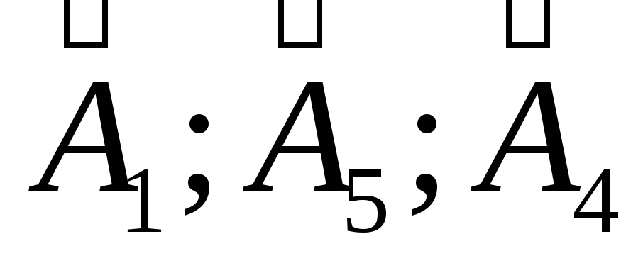 - reducing links.
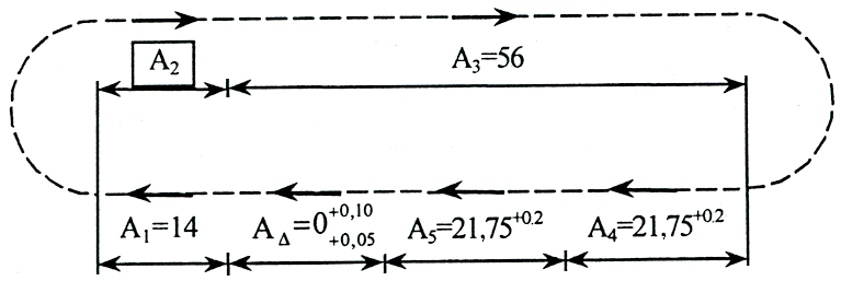
Figure 9.8 - Dimensional chain diagram
Compensator nominal size
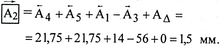
Axial play S is an axial displacement of the bearing ring from one extreme position to the other extreme position when the paired ring is stationary. The allowable S values for bearing 7210 are between 50 µm and 100 µm (table 8.4).
Thus, the dimensions of the closing link
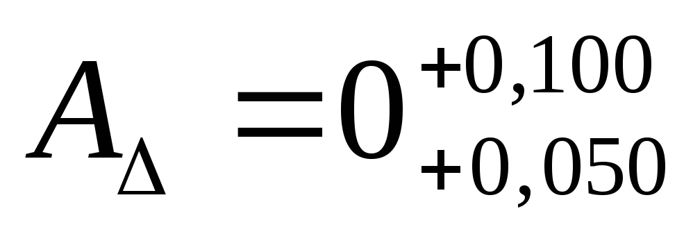 mm.
mm.
Closing link tolerance
TA ∆ = E S A ∆ - E I A ∆ = +0.1 - 0.05 = 0.05 mm = 50 μm.
We assign the manufacturing accuracy of the sizes А 1 and А 3. Let these dimensions be made according to the 10th quality. Then we have: IT 10 14 = 70 microns = 0.07 mm; IT10 56 = 120 μm = 120 mm (Table A.2).
The dimensions of links A 1 and A 3 do not apply to shafts or holes, therefore, we assign the maximum deviations to be symmetrical:
A 1 = 14 ± 0.035 mm; A 3 = 56 ± 0.060 mm;
The tolerances of links A 4 and A 5 (mounting height of bearings 7210) are known and are:
TA 4 = TA 5 = 0.2 mm.
The sum of the tolerances of the constituent links
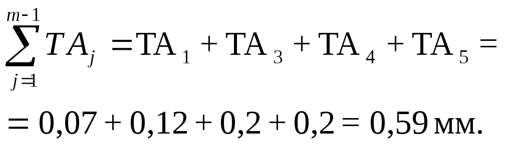
Required amount of compensation
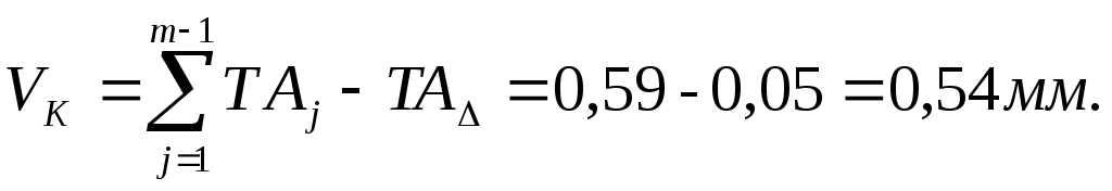
Determine the coordinate of the middle of the range V K through the coordinates of the midpoints of the tolerance fields of the links:
EcAz = 0; EcA 1 = 0; EcA 5 = + 0.1mm; EcA 4 = +0.1 mm; EcA ∆ = +0.075 mm.
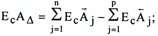
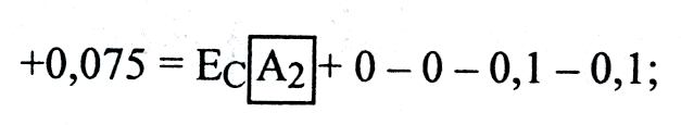
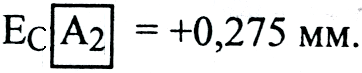
Upper and lower deflection of the compensator:
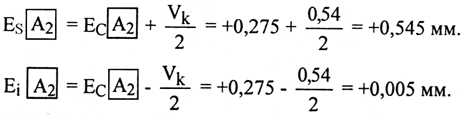
Compensator size
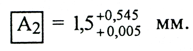
Verification calculation:
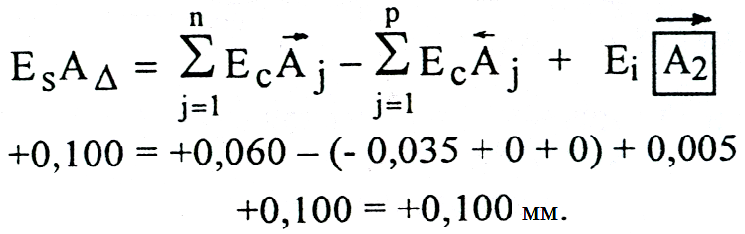
Limit dimensions of the compensator:
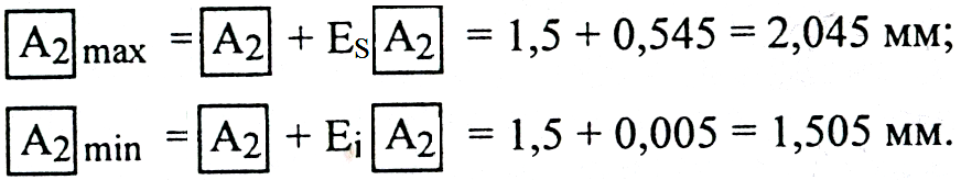
The size  can be taken as the thickness of the permanent gasket. S post = 1.505 mm.
Number of replaceable pads according to the formula:
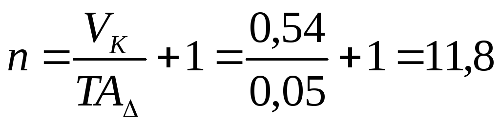 .
.
We accept n = 12 pads.
Then the thickness of the shims should be:
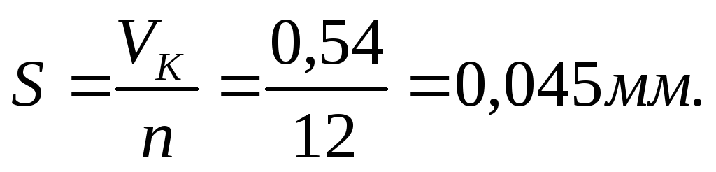
We check the calculation using the formulas:
You can accept steel tape for gaskets in accordance with GOST 503-81 with increased manufacturing accuracy (table 9.2):
S = 0.05 -0.011 mm.
Table 9.2 - Limit deviations of cold-rolled steel strip thickness from low-alloy steels (according to GOST 503 - 71)
|
Manufacturing precision |
Limit deviations, mm, with tape thickness, mm |
||||||
|
Normal | |||||||
|
Increased | |||||||
|
Note. Choose the thickness of the tape from a number of numbers: 0.05; 0.06; 0.07; 0.08; 0.09; 0.10; 0.11; 0.12; 0.15; 0.18; 0.20; 0.22; 0.25; 0.28; 0.30; 0.32; 0.35; 0.40; 0.45; 0.50; 0.55; 0.57; 0.60; 0.65; 0.70; 0.75; 0.80; 0.85; 0.90; 0.95; 1.00; 1.05; 1.10; 1.15 |
|||||||
The set of shims will consist of one permanent S post and 12 interchangeable shims. Depending on the actual dimensions of the parts, the number of gaskets will be different from the number found.
For the manufacture of gaskets, copper foil is also used in accordance with GOST 5638 - 75 (table 9.3) and brass sheets and strips in accordance with GOST 931 - 78 (table 9.4).
To reduce the number of replaceable gaskets, we can use gaskets of various thicknesses. In this case, the thickness of each subsequent gasket is taken:
 .
0,05 + 0,1 + 0,2 + 0,4 > 0,75
.
0,05 + 0,1 + 0,2 + 0,4 > 0,75
Thus, the expansion joint can have one permanent spacer 1.505 mm and four shims 0.05 mm, 0.1 mm, 0.2 mm, 0.4 mm. The final number of shims is set when assembling the assembly unit.
Table 9.3 - Copper foil roll for technical purposes (according to GOST 5638 - 75)
Table 9.4 - Brass sheets and strips (according to GOST 931 - 78)
|
Thickness, mm |
Limit deviations, mm |
Thickness, mm |
Limit deviations, mm |
|
|
Increased accuracy |
Normal Accuracy |
|||
|
1,2; 1,3; 1,35; 1,4; 1,5 | ||||
Example.
Figure 9.9 shows a low-speed gearbox shaft with the corresponding dimensions, indicated by letters with indices. The nominal value of these dimensions is taken from the drawing of a specific assembly unit. Let the nominal dimensions for this example be: A 1 = 20 mm, A 2 = 164 mm, A 3 = 20 mm, A 4 = 24 mm, A 6 = 248 mm, A 8 = 24 mm. Bearings 210.
Solution.
It is required to determine the tolerances of all constituent dimensions and the number of replaceable spacers.
Normal operating conditions of the assembly unit shown in Figure 9.9 will be possible if the axial clearances (axial play of bearings) recommended in section 8 of this work are provided for the rolling bearings.
To determine the permissible values of the axial play of the bearing 210, with the inner ring diameter d = 50 mm, according to table 8.6, we establish that the radial clearances of such a bearing can have the values g r min = 12 µm and g r max = 29 µm.
Using the nomogram in Figure 8.6, we determine the value 2S / g r. For g r min = 12 μm we find 2S / g r = 12, then the axial game 2S = 12 12 = 144 μm = 0.144 mm.
For g r max = 29 μm, we find 2S / g r = 7.2. Then the axial play 2S = 7.2 · 0.029 = 0.209 mm.
Thus, for bearing 210, the axial play can vary from 0.144 to 0.209 mm.
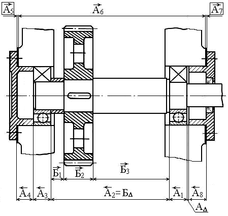
Figure 9.9 - Slow-speed gearbox shaft
We make up the main dimensional chain (Figure 9.10)
V
Figure 9.10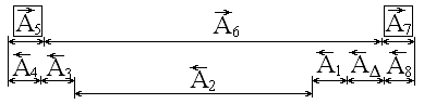
Closing link dimensions:
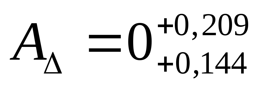 mm.
mm.
We number the links, starting from the closing link in the direction corresponding to the arrows of the increasing and decreasing links. Using the closed loop bypass method, we establish that the links A 5, A 6, A 7, increasing (lead to an increase in the size of the closing link with their growth), and all the rest - decreasing. In the considered dimensional chain, the total value  is a compensator.
Determine the nominal value of the compensator by the formula
24 + 20 + 164 + 20 + 24 – 248 = 4.
Let's distribute the amount of compensation between and:
Suppose that the gearbox parts included in this dimensional chain will be manufactured according to 11 - quality. We determine the tolerances and dimensions included in the dimensional chain in accordance with GOST 25346 - 89 (tables A.2 - A.4) and set the deviations. The permissible deviations for the width of the bearing rings (links A3, A2) are assigned in accordance with GOST 520-2002 (Table A.24).
All information about the links of the dimensional chain is summarized in table 9.5. It should be borne in mind that if the size refers to covered, then the upper limit deviation is zero, and the lower - the tolerance value, taken with a minus sign. If the size is encompassing, then its lower limit deviation is zero, and the upper one is the tolerance value, taken with a plus sign. For other sizes (not related to either female or male), the deviations are assigned symmetrical (± IT / 2).
Table 9.5
|
Link sizes |
Nominal size, mm |
The character of the link in the chain |
Upper deviation, μm |
Lower deviation, microns |
Tolerance, μm |
Notes (edit) |
|
Reducing Reducing Reducing Reducing Compensator Augmenting Compensator Reducing Closing |
GOST 520-2002 GOST 520-2002 |
Required compensation amount (Equation 9.22):
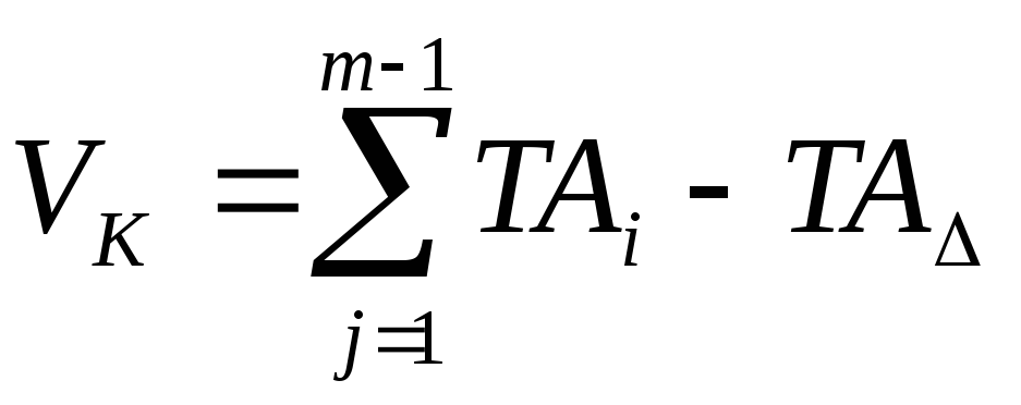 .
.
where: TA ∆ = 65 - closing link tolerance microns;
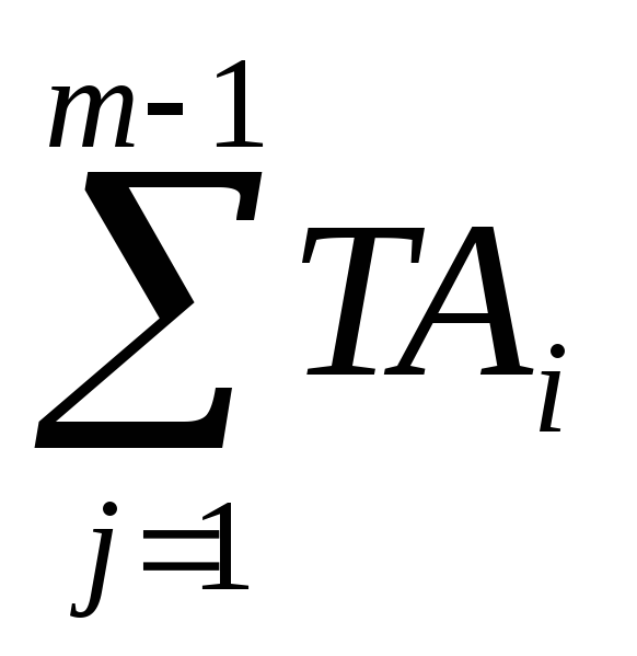 - the sum of the tolerances of the constituent links
Number of control steps (equation 9.24)
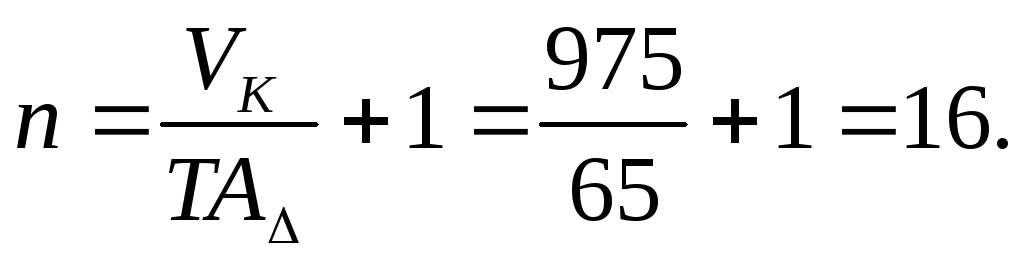
The smallest thickness of the gaskets is found by the formula 9.25
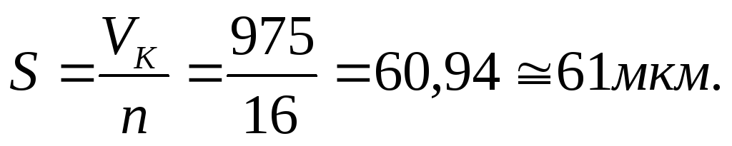
We accept the smallest thickness of the first spacer S 1 according to GOST 503-81 (table 9.2) S 1 = 0.06 mm.
Number of Replacement Shims Required (Equation 9.26)
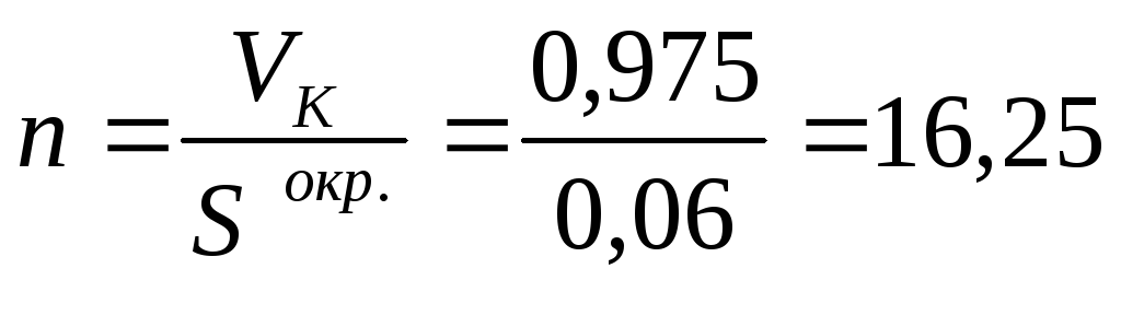
we take n = 16.
Permanent spacer
![]()
Subsequent gaskets:
The sum of the thicknesses of all shims in the set
S max ≥ V K 0.06 + 0.12 + 0.24 + 0.48 + 0.96> 0.975 μm.
Thus, the expansion joint can have one permanent spacer 3.025 mm and five shims 0.06 mm, 0.12 mm, 0.24 mm, 0.48 mm, 0.96 mm. The final number of shims is set when assembling the assembly unit.
The calculation of the derivative of the dimensional chain (Figure 9.11) is recommended to be carried out by the method of complete interchangeability. In this dimensional chain, the dimension A 2 = 164 -0.25 mm is closing, and the length of the collar B 3 = 84 mm, the width of the hub of the gear wheel B 2 = 60 mm and the width of the spacer ring B 1 = 20 mm are constituent links.
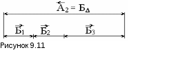
It is required to determine the tolerances and maximum deviations for all constituent links.
In view of the large difference between the nominal dimensions of the constituent links, the calculation should be applied by the method of one accuracy grade.
When using the method of one quality of accuracy, we determine the average number of tolerance units in the dimensional chain according to the formula (9.18)
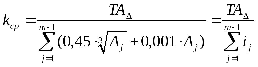
By the number of tolerance units, the required quality is determined according to table 3.2
The values 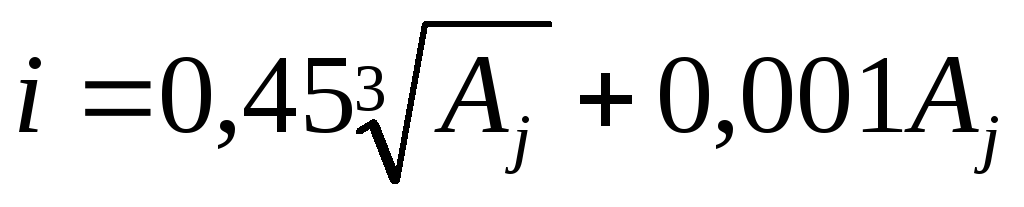 can be taken according to table 9.6.
Table 9.6
|
Size intervals, mm Above - up to | ||||||||||||
|
I-value, μm |
For the derived dimensional chain of the example under consideration:
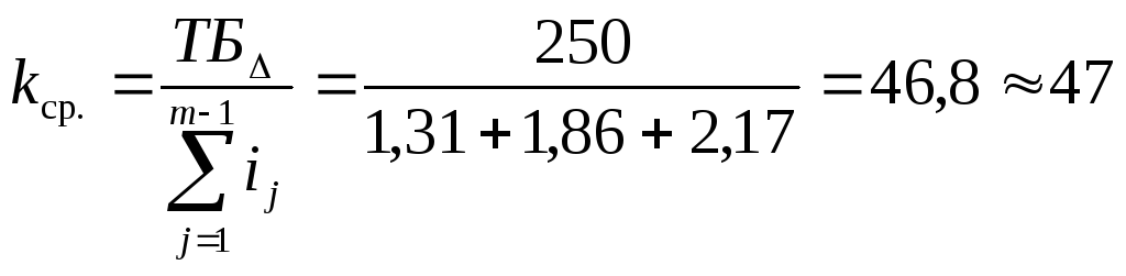
According to table 3.2, we determine that the obtained value of the tolerance unit k is between 9 and 10 grades. Therefore, part of the links of the dimensional chain can be made according to grade 9, and part to grade 10.
As a result, for the indicated nominal sizes and the qualities found according to table A2, we have:
IT9 60 = 74 μm; IT9 84 = 87 μm; IT10 20 = 84 μm.
Dimensions of links with deviations:
B 2 = 60 -0.074 mm; B 3 = 84 -0.087 mm; B 1 = 20 -0.084 mm.
If standard tolerances are assigned to chain links (without correction), then it is permissible that 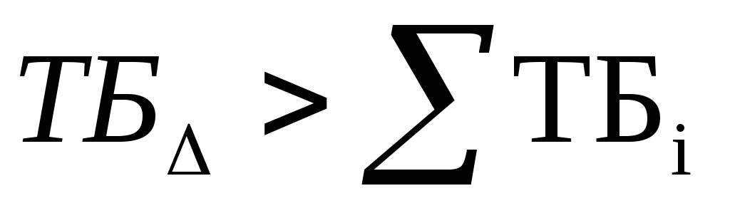 by (5 ... 6)%.
- Complete biography of L.N. Tolstoy: life and work. Interesting facts from the life of fat Leo Tolstoy short biography teacher
- Report: Tolstoy Lev Nikolaevich Small biography of Tolstoy
- After the "Thunderstorms Message about the play Thunderstorm
- The history of the creation of the play "The Thunderstorm" by Ostrovsky Where the drama of the Ostrovsky thunderstorm takes place